Overview
Frequency tables are one of the most fundamental tools in data analysis and statistics, representing a systematic way to organize and display data by showing how often each value or category appears in a dataset. On the GRE Quantitative Reasoning section, gre frequency tables appear regularly in Data Interpretation questions, often combined with other statistical concepts such as mean, median, mode, range, and percentiles. These tables condense raw data into an easily interpretable format, allowing test-takers to quickly extract information and perform calculations that would be cumbersome with unorganized data.
Understanding frequency tables is essential for GRE success because they form the foundation for more complex statistical reasoning. The GRE frequently presents data in tabular format, and students must be able to read these tables accurately, identify patterns, calculate summary statistics, and draw valid conclusions under time pressure. Questions involving frequency tables often test multiple skills simultaneously: reading comprehension of tabular data, arithmetic calculations, proportional reasoning, and logical inference. Mastery of this topic directly impacts performance on approximately 15-20% of Quantitative Reasoning questions, particularly in the Data Interpretation sets that appear in every GRE exam.
Frequency tables connect to broader Quantitative Reasoning concepts including probability (where frequencies determine likelihood), descriptive statistics (where tables provide the raw material for calculating measures of central tendency and spread), and data visualization (where tables often accompany or replace graphs and charts). The ability to work fluently with frequency tables also supports success in questions involving weighted averages, percentile calculations, and comparative data analysis—all high-yield GRE question types.
Learning Objectives
- [ ] Identify when Frequency tables is being tested
- [ ] Explain the core rule or strategy behind Frequency tables
- [ ] Apply Frequency tables to GRE-style questions accurately
- [ ] Calculate measures of central tendency (mean, median, mode) directly from frequency tables
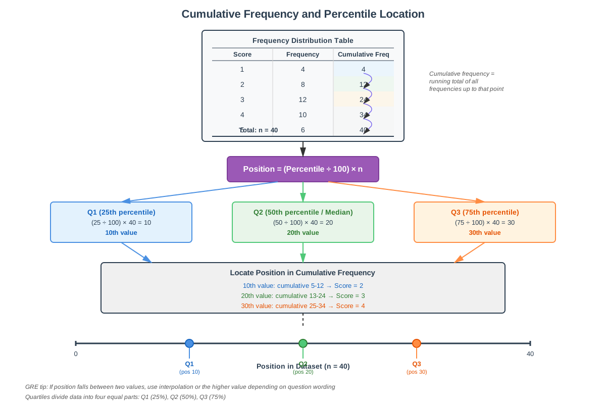
- [ ] Determine cumulative frequencies and use them to find percentiles and quartiles
- [ ] Construct frequency tables from raw data or verbal descriptions
- [ ] Recognize and interpret both simple and grouped frequency distributions
Prerequisites
- Basic arithmetic operations: Essential for calculating totals, products, and sums when working with frequencies and values
- Understanding of mean, median, and mode: Frequency tables are tools for organizing data to calculate these measures efficiently
- Fraction and percentage calculations: Many frequency table questions require converting between counts, fractions, and percentages
- Basic algebraic manipulation: Needed when frequency tables contain variables or when solving for unknown values
Why This Topic Matters
Frequency tables represent one of the most practical statistical tools used across disciplines—from business analytics and scientific research to public policy and healthcare. In real-world applications, frequency tables help organizations understand customer behavior patterns, researchers analyze experimental results, and policymakers interpret demographic data. The ability to quickly organize, interpret, and extract insights from tabular data is a fundamental skill in data-driven decision-making.
On the GRE, frequency tables appear in approximately 3-5 questions per exam, making them a high-yield topic for focused study. They most commonly appear in Data Interpretation sets (those multi-question sets based on graphs or tables), but also surface in individual Quantitative Comparison and Problem Solving questions. The ETS (Educational Testing Service) favors frequency tables because they efficiently test multiple competencies: numerical reasoning, attention to detail, calculation accuracy, and the ability to synthesize information from structured data.
Common exam presentations include: tables showing test score distributions and asking for percentile calculations; tables displaying survey results requiring percentage or ratio comparisons; tables with missing values that must be determined from given constraints; and tables paired with other data visualizations (bar graphs, pie charts) where students must reconcile information across multiple representations. The GRE particularly favors questions that require multi-step reasoning, such as calculating a weighted average from a frequency distribution or determining how many data points fall within a specific range.
Core Concepts
Definition and Structure of Frequency Tables
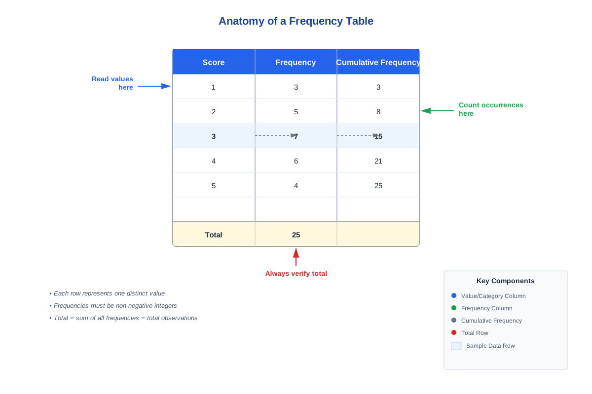
A frequency table (also called a frequency distribution) is a systematic arrangement of data values alongside their corresponding frequencies—the number of times each value appears in a dataset. The basic structure consists of at least two columns: one listing the distinct data values or categories, and another showing how many times each value occurs. The frequency of a value represents its count or occurrence in the dataset.
For example, if a dataset contains test scores {85, 90, 85, 75, 90, 85, 80}, a frequency table would organize this as:
| Score | Frequency |
|---|---|
| 75 | 1 |
| 80 | 1 |
| 85 | 3 |
| 90 | 2 |
The sum of all frequencies always equals the total number of data points (in this case, 7). This fundamental property serves as a check for accuracy when constructing or interpreting frequency tables.
Types of Frequency Tables
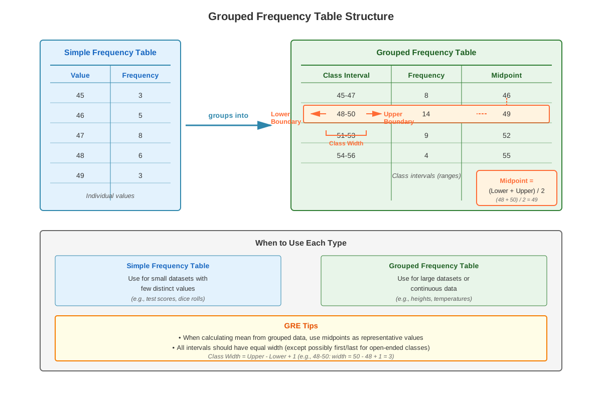
Simple frequency tables list individual values with their frequencies, as shown above. These work well when the dataset contains a limited number of distinct values. Grouped frequency tables (or class interval tables) organize data into ranges or intervals, particularly useful when dealing with continuous data or large datasets with many distinct values.
For grouped tables, data is organized into class intervals or bins:
| Score Range | Frequency |
|---|---|
| 70-79 | 2 |
| 80-89 | 4 |
| 90-99 | 3 |
When working with grouped frequency tables, the class midpoint (the average of the lower and upper boundaries) often represents the entire interval for calculation purposes. For the interval 70-79, the midpoint is 74.5.
Cumulative Frequency
Cumulative frequency represents the running total of frequencies up to and including a particular value or class. It answers the question: "How many data points are less than or equal to this value?" Cumulative frequency is calculated by adding each frequency to the sum of all previous frequencies.
| Score | Frequency | Cumulative Frequency |
|---|---|---|
| 75 | 1 | 1 |
| 80 | 1 | 2 |
| 85 | 3 | 5 |
| 90 | 2 | 7 |
Cumulative frequencies are essential for determining percentiles, quartiles, and medians. The median, for instance, is the value at the cumulative frequency position of (n+1)/2, where n is the total number of data points.
Relative Frequency and Percentage Frequency
Relative frequency expresses each frequency as a proportion of the total, calculated by dividing the individual frequency by the sum of all frequencies. Percentage frequency is simply relative frequency multiplied by 100.
| Score | Frequency | Relative Frequency | Percentage Frequency |
|---|---|---|---|
| 75 | 1 | 1/7 ≈ 0.143 | 14.3% |
| 80 | 1 | 1/7 ≈ 0.143 | 14.3% |
| 85 | 3 | 3/7 ≈ 0.429 | 42.9% |
| 90 | 2 | 2/7 ≈ 0.286 | 28.6% |
These representations are particularly useful for comparing datasets of different sizes or for probability calculations, where relative frequency approximates probability.
Calculating Statistics from Frequency Tables
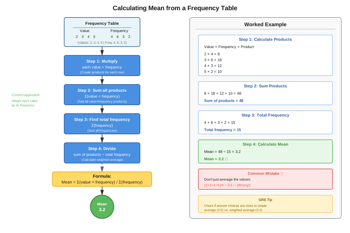
Frequency tables enable efficient calculation of summary statistics without listing every individual data point. The mean from a frequency table is calculated using the formula:
Mean = (Σ(value × frequency)) / (Σfrequency)For the example above: Mean = (75×1 + 80×1 + 85×3 + 90×2) / 7 = (75 + 80 + 255 + 180) / 7 = 590 / 7 ≈ 84.3
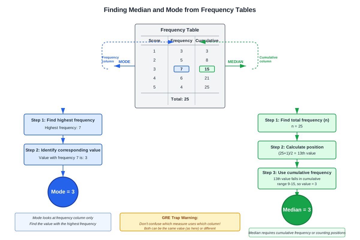
The mode is the value with the highest frequency (85 in this example). The median is found by locating the middle position using cumulative frequency. With 7 data points, the median is at position 4, which falls in the cumulative frequency range for score 85.
Reading and Interpreting Frequency Tables
Effective interpretation requires attention to several elements: the table title (which provides context), column headers (which specify what data is being presented), units of measurement, and any footnotes or legends. On the GRE, questions often test whether students notice important details such as whether frequencies represent counts or percentages, whether all categories are shown or if there's an "other" category, and whether the data represents a sample or a population.
Concept Relationships
Frequency tables serve as the organizational foundation that connects raw data to statistical analysis. The relationship flows as follows: Raw Data → Frequency Table → Summary Statistics → Interpretation and Decision-Making. The frequency table acts as an intermediary structure that makes complex datasets manageable and calculations feasible.
Within the topic itself, simple frequency tables lead to cumulative frequency tables, which enable percentile and quartile calculations. Relative frequency connects frequency tables to probability theory, as the relative frequency of an event approximates its probability in large samples. Grouped frequency tables extend the concept to handle continuous or extensive data, introducing the additional concept of class intervals and midpoints.
Frequency tables connect backward to prerequisite topics: arithmetic operations provide the computational tools, while understanding of mean, median, and mode gives purpose to the organization. They connect forward to more advanced topics including probability distributions (where frequency tables represent discrete probability distributions), hypothesis testing (where observed frequencies are compared to expected frequencies), and data visualization (where frequency tables provide the numerical basis for histograms, bar charts, and frequency polygons).
The relationship can be mapped as: Basic Counting → Frequency Tables → Cumulative Frequency → Percentiles/Quartiles → Box Plots and Distribution Analysis. Similarly: Frequency Tables → Relative Frequency → Probability → Expected Value Calculations.
High-Yield Facts
⭐ The sum of all frequencies in a frequency table always equals the total number of observations in the dataset
⭐ The mode is the value with the highest frequency; a dataset can have multiple modes or no mode
⭐ To calculate the mean from a frequency table: multiply each value by its frequency, sum these products, then divide by the total frequency
⭐ Cumulative frequency at any point equals the sum of all frequencies up to and including that point
⭐ The median position in a dataset of n values is at (n+1)/2; use cumulative frequency to locate this position
- Relative frequency = (individual frequency) / (total frequency); it always falls between 0 and 1
- Percentage frequency = relative frequency × 100; all percentage frequencies sum to 100%
- In grouped frequency tables, the class midpoint is used to represent all values in that interval for calculation purposes
- The range of a dataset can be determined from a frequency table by subtracting the smallest value from the largest value
- When a frequency table shows "n" as the total, you may need to use given information to solve for n before performing other calculations
- Frequency tables can represent both categorical data (colors, brands, categories) and numerical data (scores, ages, measurements)
- The class with the highest frequency in a grouped frequency table is called the modal class
Quick check — test yourself on Frequency tables so far.
Try Flashcards →Common Misconceptions
Misconception: The mode is always the middle value in a frequency table → Correction: The mode is the value with the highest frequency, regardless of its position in the table. A value appearing once at the top of the table could be the mode if all other values have frequency zero, though this would be unusual.
Misconception: To find the median, simply locate the middle row of the frequency table → Correction: The median is the middle value when all data points are arranged in order. You must use cumulative frequency to determine which value corresponds to the middle position. A value in the first row could be the median if its frequency is large enough.
Misconception: Mean equals the sum of the values shown in the frequency table divided by the number of rows → Correction: Mean equals the sum of (each value multiplied by its frequency) divided by the total frequency. Each value must be weighted by how many times it appears.
Misconception: If a frequency table shows percentages, you cannot calculate the actual number of observations → Correction: If you're given the total number of observations (n) or can determine it from context, you can convert percentages back to frequencies by multiplying by n and dividing by 100.
Misconception: Cumulative frequency and frequency are the same thing → Correction: Frequency shows how many times a specific value appears; cumulative frequency shows how many observations are less than or equal to that value. Cumulative frequency is always greater than or equal to the individual frequency and increases monotonically down the table.
Misconception: In grouped frequency tables, all values in an interval are equal to the lower boundary → Correction: Values in an interval are distributed throughout that range. For calculations, the class midpoint (average of lower and upper boundaries) is typically used to represent the interval, though this is an approximation.
Worked Examples
Example 1: Calculating Statistics from a Simple Frequency Table
Problem: The following frequency table shows the number of hours students studied for an exam:
| Hours Studied | Frequency |
|---|---|
| 2 | 3 |
| 3 | 5 |
| 4 | 7 |
| 5 | 4 |
| 6 | 1 |
(a) What is the mean number of hours studied?
(b) What is the median number of hours studied?
(c) What percentage of students studied 4 or more hours?
Solution:
(a) To find the mean, calculate Σ(value × frequency) / Σfrequency:
- Total frequency: 3 + 5 + 7 + 4 + 1 = 20 students
- Sum of (value × frequency): (2×3) + (3×5) + (4×7) + (5×4) + (6×1) = 6 + 15 + 28 + 20 + 6 = 75
- Mean = 75 / 20 = 3.75 hours
(b) To find the median with 20 observations, we need the average of the 10th and 11th values:
- Create cumulative frequency: 3, 8, 15, 19, 20
- The 10th value falls in the cumulative frequency of 15 (corresponding to 4 hours)
- The 11th value also falls in the cumulative frequency of 15 (corresponding to 4 hours)
- Median = 4 hours
(c) Students who studied 4 or more hours: 7 + 4 + 1 = 12 students
- Percentage = (12/20) × 100 = 60%
This example demonstrates the core learning objectives of applying frequency table concepts to calculate multiple statistics and interpreting the results accurately.
Example 2: Working with Grouped Frequency Tables and Missing Information
Problem: A survey recorded the ages of participants in a fitness program. The grouped frequency table is partially complete:
| Age Range | Frequency | Cumulative Frequency |
|---|---|---|
| 20-29 | 8 | 8 |
| 30-39 | 12 | 20 |
| 40-49 | x | 35 |
| 50-59 | 10 | 45 |
| 60-69 | 5 | 50 |
(a) What is the value of x?
(b) Estimate the mean age using class midpoints.
(c) In which age range does the median fall?
Solution:
(a) From the cumulative frequency column:
- At age range 40-49, cumulative frequency is 35
- At age range 30-39, cumulative frequency is 20
- Therefore, x = 35 - 20 = 15
(b) Using class midpoints (24.5, 34.5, 44.5, 54.5, 64.5):
- Sum of (midpoint × frequency): (24.5×8) + (34.5×12) + (44.5×15) + (54.5×10) + (64.5×5)
- = 196 + 414 + 667.5 + 545 + 322.5 = 2,145
- Total frequency = 50
- Estimated mean = 2,145 / 50 = 42.9 years
(c) With 50 observations, the median is at position (50+1)/2 = 25.5 (average of 25th and 26th values):
- Looking at cumulative frequency, position 25.5 falls between cumulative frequency 20 and 35
- Therefore, the median falls in the age range 40-49
This example illustrates how to work with incomplete information, use grouped data for calculations, and apply cumulative frequency to locate the median position—all common GRE question types.
Exam Strategy
When approaching GRE questions involving frequency tables, begin by quickly scanning the table structure to identify: (1) what the rows and columns represent, (2) whether frequencies are given as counts or percentages, (3) the total number of observations, and (4) whether any cumulative frequency information is provided or needs to be calculated.
Trigger words and phrases that signal frequency table questions include: "the table shows," "distribution of," "how many," "what percentage," "median value," "most common," "average of," and "cumulative." Questions asking for "the number of observations" or "how many data points" require summing frequencies, while questions about "proportion" or "percentage" require calculating relative frequencies.
For process of elimination, immediately eliminate answer choices that: (1) exceed the total frequency when the question asks "how many," (2) fall outside the range of values shown in the table, (3) represent impossible percentages (negative or greater than 100%), or (4) contradict basic properties (such as a median that's larger than all values in the table).
Time allocation strategy: Simple frequency table questions should take 1-1.5 minutes, while complex multi-step problems involving grouped frequencies or multiple calculations may require 2-2.5 minutes. If a Data Interpretation set includes a frequency table, budget approximately 1 minute per question but be prepared to spend slightly more on the first question as you familiarize yourself with the table structure.
Exam Tip: Always verify that your calculated frequencies sum to the given total. This simple check catches arithmetic errors and ensures you haven't misread the table.
Create a quick cumulative frequency column in your scratch work if the question involves median, percentiles, or phrases like "at least," "no more than," or "between." This small time investment (15-20 seconds) often saves time and prevents errors on subsequent calculations.
Memory Techniques
MNEMONIC for calculating mean from frequency tables: "VFT" - Value times Frequency, then Total
- Multiply each Value by its Frequency
- Sum these products
- Divide by Total frequency
MNEMONIC for frequency table components: "VFCR" - Values, Frequencies, Cumulative, Relative
- This reminds you of the four main columns you might encounter or need to construct
Visualization strategy: Picture a frequency table as a "collapsed" list of data. Each frequency tells you how many times to "expand" that value. For example, a frequency of 5 for the value 10 means five 10s in the original dataset: [10, 10, 10, 10, 10].
Acronym for checking work: "STAR" - Sum frequencies (should equal total), Test extreme values (do they make sense?), Assess units (counts vs. percentages), Review calculations (especially multiplication)
For remembering the median position formula: "N plus one, divided by two, finds the middle for you" - Position = (n+1)/2
To remember that mode = highest frequency: "Mode is Most" - the value that appears the MOST frequently
Summary
Frequency tables are essential organizational tools that systematically display how often each value or category appears in a dataset. Mastery of frequency tables requires understanding their structure (values paired with frequencies), recognizing different types (simple vs. grouped), and efficiently calculating summary statistics including mean (sum of value×frequency divided by total frequency), median (using cumulative frequency to locate the middle position), and mode (value with highest frequency). Cumulative frequency, which represents running totals, enables percentile and quartile calculations. Relative and percentage frequencies express proportions and facilitate comparisons across datasets. On the GRE, frequency table questions test multiple skills simultaneously: accurate table reading, arithmetic calculation, statistical reasoning, and logical inference. Success requires attention to detail (distinguishing counts from percentages, noting all categories), systematic calculation methods (creating cumulative frequency columns when needed), and verification strategies (ensuring frequencies sum correctly). The ability to quickly extract information from frequency tables and perform multi-step calculations accurately is fundamental to achieving high scores on GRE Data Interpretation questions.
Key Takeaways
- Frequency tables organize data by showing how many times each value appears; the sum of all frequencies equals the total number of observations
- Calculate mean from a frequency table by finding Σ(value × frequency) / Σfrequency, not by averaging the values shown
- Use cumulative frequency to locate the median position at (n+1)/2 and to answer questions about "at least" or "no more than" a certain value
- The mode is the value with the highest frequency, which may appear anywhere in the table and may not be unique
- Relative frequency (individual frequency ÷ total frequency) converts counts to proportions and connects frequency tables to probability
- In grouped frequency tables, use class midpoints to represent intervals when calculating statistics like the mean
- Always verify that calculated frequencies sum to the given total as a check for arithmetic accuracy
Related Topics
Measures of Central Tendency and Spread: Building on frequency tables, this topic explores mean, median, mode, range, variance, and standard deviation in greater depth, including how to calculate these measures efficiently from various data representations.
Percentiles and Quartiles: Extends cumulative frequency concepts to divide datasets into meaningful segments, essential for understanding box plots and comparing individual values to group distributions.
Probability Distributions: Frequency tables represent discrete probability distributions when converted to relative frequencies, forming the foundation for understanding probability concepts tested on the GRE.
Data Visualization: Frequency tables provide the numerical foundation for creating and interpreting histograms, bar charts, and frequency polygons—all common GRE question formats.
Weighted Averages: Many GRE questions combine frequency table concepts with weighted average calculations, where frequencies serve as weights for different values.
Practice CTA
Now that you've mastered the fundamentals of frequency tables, it's time to solidify your understanding through active practice. Attempt the practice questions to apply these concepts under exam-like conditions, and use the flashcards to reinforce key definitions and formulas. Remember, frequency tables appear in approximately 15-20% of GRE Quantitative Reasoning questions—your investment in mastering this topic will directly translate to points on test day. Focus on accuracy first, then build speed as the concepts become automatic. You've got this!
Sign up free to keep reading
Create a free AnvayaPrep account to finish this GRE guide on Frequency tables — plus flashcards and practice questions.