Overview
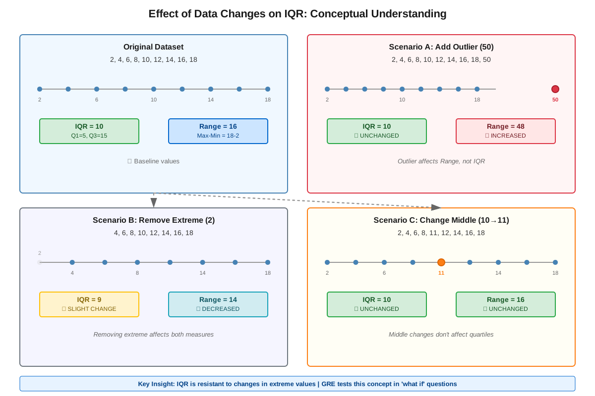
The interquartile range (IQR) is a fundamental measure of statistical dispersion that quantifies the spread of the middle 50% of a dataset. Unlike the range, which considers only the extreme values, the IQR focuses on the central portion of data by measuring the distance between the first quartile (Q1) and the third quartile (Q3). This makes it particularly robust against outliers and extreme values, which is why the GRE interquartile range questions frequently appear in Data Analysis sections to test students' understanding of data variability and distribution characteristics.
On the GRE Quantitative Reasoning section, understanding the interquartile range is essential because it appears in multiple question formats: quantitative comparison questions, data interpretation sets, and problem-solving questions involving box plots or statistical analysis. The GRE tests not only computational ability but also conceptual understanding of when and why the IQR provides more meaningful information than other measures of spread. Questions may ask students to calculate the IQR directly, compare it across different datasets, or interpret its meaning in context.
The interquartile range connects to broader statistical concepts including measures of central tendency (mean, median, mode), other measures of dispersion (range, standard deviation), and data visualization techniques (box plots, histograms). Mastering the IQR enables students to analyze data distributions more comprehensively, identify outliers systematically, and make informed comparisons between datasets—all critical skills for achieving a competitive score on the GRE Quantitative Reasoning section.
Learning Objectives
- [ ] Identify when Interquartile range is being tested in GRE questions
- [ ] Explain the core rule or strategy behind Interquartile range calculations
- [ ] Apply Interquartile range to GRE-style questions accurately
- [ ] Calculate quartiles (Q1, Q2, Q3) for both odd and even-numbered datasets
- [ ] Interpret the meaning of IQR values in context and compare spread across multiple datasets
- [ ] Recognize how outliers affect IQR versus other measures of dispersion
- [ ] Construct and interpret box plots using quartile information
Prerequisites
- Basic arithmetic operations: Essential for calculating quartile positions and performing subtraction to find the IQR
- Understanding of median: The median concept directly extends to quartiles, as Q2 is the median of the entire dataset
- Ordered data sets: Ability to arrange numbers in ascending order, which is required before identifying quartiles
- Percentiles concept: Quartiles are specific percentiles (25th, 50th, 75th), so understanding percentile ranking aids comprehension
- Basic set notation: Familiarity with representing and manipulating numerical datasets
Why This Topic Matters
The interquartile range serves as a critical tool in real-world data analysis across numerous fields. Researchers use IQR to identify outliers in experimental data, financial analysts employ it to assess investment risk and volatility, and quality control specialists apply it to detect manufacturing defects. In educational assessment, IQR helps evaluate score distributions and identify performance gaps. Medical researchers rely on IQR when dealing with skewed health data where extreme values might distort other statistical measures.
On the GRE, interquartile range questions appear with moderate to high frequency, typically comprising 1-3 questions per exam administration. These questions most commonly appear in Data Interpretation sets (where students analyze charts, tables, or graphs), quantitative comparison questions (comparing IQR values across datasets), and problem-solving questions involving box plots. The GRE particularly favors questions that test conceptual understanding rather than pure computation—for instance, asking how adding or removing data points affects the IQR, or which measure of spread (IQR versus range versus standard deviation) is most appropriate for a given scenario.
The exam commonly presents IQR in several contexts: analyzing salary distributions where outliers exist, comparing test score variability across different groups, interpreting box plots showing multiple data distributions, and evaluating the effect of data transformations on spread measures. Questions may also integrate IQR with other statistical concepts, requiring students to understand relationships between quartiles, percentiles, and measures of central tendency.
Core Concepts
Definition and Formula
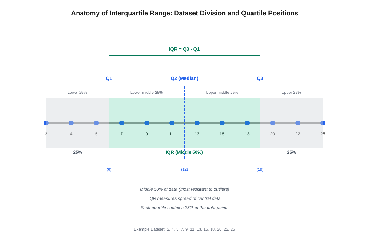
The interquartile range is defined as the difference between the third quartile (Q3) and the first quartile (Q1) of a dataset. Mathematically:
IQR = Q3 - Q1This measure captures the range of the middle 50% of the data, effectively eliminating the influence of the lowest 25% and highest 25% of values. The IQR represents the spread of data around the median, making it a measure of statistical dispersion that is resistant to outliers.
Understanding Quartiles
Quartiles divide an ordered dataset into four equal parts, each containing approximately 25% of the data points:
- Q1 (First Quartile): The median of the lower half of the data; 25% of values fall below Q1
- Q2 (Second Quartile): The median of the entire dataset; 50% of values fall below Q2
- Q3 (Third Quartile): The median of the upper half of the data; 75% of values fall below Q3
The relationship between quartiles and percentiles is direct: Q1 corresponds to the 25th percentile, Q2 to the 50th percentile, and Q3 to the 75th percentile.
Calculating Quartiles: Step-by-Step Process
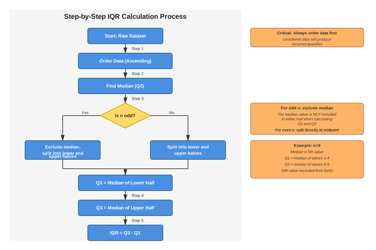
Step 1: Order the data
Arrange all values in ascending order from smallest to largest.
Step 2: Find the median (Q2)
- If n (number of values) is odd: Q2 is the middle value
- If n is even: Q2 is the average of the two middle values
Step 3: Divide the dataset
- Lower half: All values below Q2 (excluding Q2 if n is odd)
- Upper half: All values above Q2 (excluding Q2 if n is odd)
Step 4: Find Q1
Calculate the median of the lower half using the same method as Step 2.
Step 5: Find Q3
Calculate the median of the upper half using the same method as Step 2.
Step 6: Calculate IQR
Subtract Q1 from Q3.
Alternative Method: Position Formula
For datasets where precise positions are needed, use the position formula:
- Q1 position = 0.25(n + 1)
- Q3 position = 0.75(n + 1)
If the position is not a whole number, interpolate between the two adjacent values. For example, if Q1 position = 3.5, take the average of the 3rd and 4th values.
Properties of the Interquartile Range
| Property | Description | Implication |
|---|---|---|
| Outlier Resistance | IQR is not affected by extreme values | More reliable than range for skewed distributions |
| Scale Dependence | IQR changes proportionally with data scaling | Multiplying all values by k multiplies IQR by k |
| Translation Invariance | Adding a constant to all values doesn't change IQR | IQR measures spread, not location |
| Non-negative | IQR ≥ 0 always | Zero IQR indicates no variability in middle 50% |
| Unit Preservation | IQR has same units as original data | Facilitates interpretation in context |
Box Plots and the Five-Number Summary
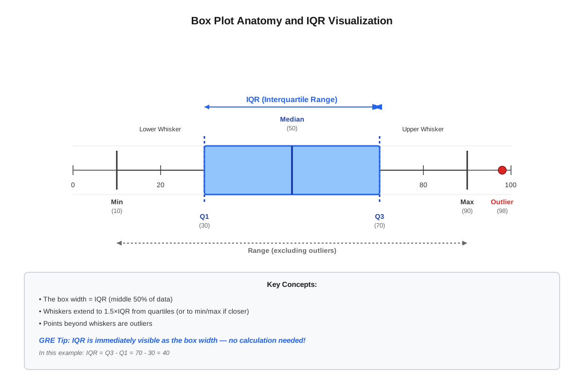
The interquartile range is visually represented in box plots (also called box-and-whisker plots), which display the five-number summary:
- Minimum value
- Q1 (bottom of box)
- Q2/Median (line inside box)
- Q3 (top of box)
- Maximum value
The box itself represents the IQR, with its height equal to the IQR value. The "whiskers" extend to the minimum and maximum values (or to defined boundaries when outliers are present). This visualization makes comparing spread across multiple datasets intuitive and immediate.
Outlier Detection Using IQR
The IQR provides a systematic method for identifying outliers:
- Lower boundary: Q1 - 1.5(IQR)
- Upper boundary: Q3 + 1.5(IQR)
Any value below the lower boundary or above the upper boundary is considered a potential outlier. This 1.5×IQR rule is widely used in statistical analysis and is the standard method for determining outliers in box plots.
Comparing IQR with Other Measures of Spread
Understanding when to use IQR versus other dispersion measures is crucial for GRE success:
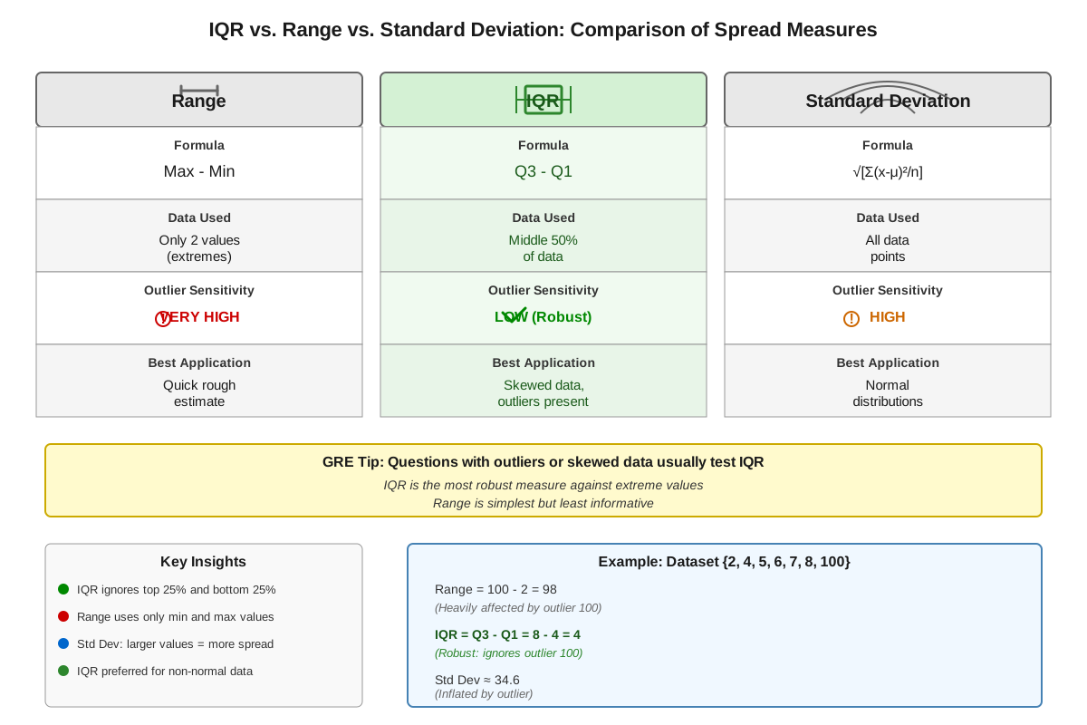
| Measure | Calculation | Advantages | Disadvantages | Best Used When |
|---|---|---|---|---|
| Range | Max - Min | Simple, intuitive | Extremely sensitive to outliers | Data has no outliers |
| IQR | Q3 - Q1 | Outlier-resistant, robust | Ignores 50% of data | Outliers present or skewed data |
| Standard Deviation | √[Σ(x-μ)²/n] | Uses all data points | Sensitive to outliers | Normal distribution, no outliers |
| Variance | Σ(x-μ)²/n | Mathematical properties | Units are squared | Theoretical calculations |
Concept Relationships
The interquartile range exists within a hierarchical structure of statistical concepts. At the foundation, ordered datasets are required before any quartile calculations can occur. The concept of median directly extends to quartiles, as finding Q1 and Q3 involves calculating medians of data subsets. The median itself is Q2, creating an intrinsic connection between these measures.
The relationship flows as follows: Ordered Data → Median (Q2) → Q1 and Q3 → IQR. Each step builds upon the previous, making the median calculation prerequisite knowledge for understanding quartiles.
The IQR connects horizontally to other measures of dispersion (range, standard deviation, variance), all of which quantify data spread but with different sensitivities to outliers and different computational approaches. The IQR's outlier resistance makes it complementary to the range—when these two measures differ substantially, outliers are likely present.
Vertically, the IQR connects to data visualization through box plots, which graphically represent the five-number summary. Understanding IQR enables interpretation of box plot dimensions and comparisons across multiple distributions. The IQR also connects to outlier detection, as the 1.5×IQR rule provides a standardized method for identifying extreme values.
Finally, the IQR relates to percentiles as a special case: Q1 is the 25th percentile, Q3 is the 75th percentile, and the IQR represents the span between these percentile markers. This connection helps students understand that quartiles are simply specific percentile divisions of the data.
High-Yield Facts
⭐ The interquartile range equals Q3 minus Q1, representing the spread of the middle 50% of data
⭐ IQR is resistant to outliers, making it superior to range for skewed distributions
⭐ To find quartiles, first order the data, then find the median, then find medians of each half
⭐ The box in a box plot has height equal to the IQR
⭐ Outliers are defined as values beyond Q1 - 1.5(IQR) or Q3 + 1.5(IQR)
- Adding the same constant to every data value does not change the IQR
- Multiplying every data value by a constant k multiplies the IQR by |k|
- An IQR of zero indicates that at least 50% of the data values are identical
- Q2 (the median) is not used in calculating IQR, though it's found during the process
- For small datasets (n < 10), different calculation methods may yield slightly different quartile values
- The IQR contains exactly 50% of the data points in the distribution
- A larger IQR indicates greater variability in the central portion of the data
- The IQR can be used to compare spread across datasets with different units by calculating the coefficient of quartile deviation
Quick check — test yourself on Interquartile range so far.
Try Flashcards →Common Misconceptions
Misconception: The IQR includes the median (Q2) in its calculation.
Correction: The IQR is calculated as Q3 - Q1 only. While Q2 is found during the process of determining quartiles, it does not appear in the IQR formula itself. The IQR measures the spread between the first and third quartiles exclusively.
Misconception: The IQR represents 50% of the data values numerically.
Correction: The IQR represents the range (spread) that contains the middle 50% of data points, not 50% of the sum of values. It's a measure of dispersion, not a proportion of the total numerical value.
Misconception: Outliers always change the IQR significantly.
Correction: The IQR is specifically designed to be resistant to outliers. Extreme values in the lowest 25% or highest 25% of data do not affect Q1 or Q3, and therefore don't change the IQR. This outlier resistance is the IQR's primary advantage over the range.
Misconception: A larger dataset always has a larger IQR.
Correction: The IQR measures spread, not dataset size. A small dataset can have a large IQR if its middle values are widely dispersed, while a large dataset can have a small IQR if its middle values are tightly clustered. Dataset size (n) and IQR are independent properties.
Misconception: When calculating quartiles, always include the median in both halves of the data.
Correction: For datasets with an odd number of values, the median should be excluded when dividing the data into lower and upper halves. Including it in both halves would incorrectly weight the center of the distribution. For even-numbered datasets, this issue doesn't arise since the median falls between two values.
Misconception: The IQR and range measure the same thing with different formulas.
Correction: While both measure spread, they capture fundamentally different aspects. The range measures total spread (including outliers), while the IQR measures spread of the central data (excluding extremes). They serve different analytical purposes and can lead to different conclusions about data variability.
Misconception: Doubling all values in a dataset doubles the IQR.
Correction: This is actually TRUE, not a misconception. However, students often incorrectly believe that adding a constant doubles the IQR. To clarify: multiplying by k multiplies IQR by |k|, but adding a constant leaves IQR unchanged.
Worked Examples
Example 1: Basic IQR Calculation
Problem: Calculate the interquartile range for the following test scores: 72, 85, 91, 68, 77, 95, 88, 73, 82, 79, 84
Solution:
Step 1: Order the data
68, 72, 73, 77, 79, 82, 84, 85, 88, 91, 95
Step 2: Find the median (Q2)
With n = 11 (odd), the median is the 6th value: Q2 = 82
Step 3: Divide the dataset
- Lower half (excluding median): 68, 72, 73, 77, 79
- Upper half (excluding median): 84, 85, 88, 91, 95
Step 4: Find Q1
The lower half has 5 values, so Q1 is the 3rd value: Q1 = 73
Step 5: Find Q3
The upper half has 5 values, so Q3 is the 3rd value: Q3 = 88
Step 6: Calculate IQR
IQR = Q3 - Q1 = 88 - 73 = 15
Interpretation: The middle 50% of test scores span 15 points, indicating moderate variability in the central portion of the distribution. This IQR value helps us understand that most students scored within a 15-point range around the median.
Connection to Learning Objectives: This example demonstrates the core calculation strategy and applies the step-by-step process to a GRE-style dataset.
Example 2: Comparing Datasets and Identifying Outliers
Problem: Two classes took the same exam. Class A scores: 65, 70, 72, 75, 78, 80, 82, 85, 88, 92. Class B scores: 45, 73, 75, 77, 78, 79, 81, 83, 85, 98. Calculate the IQR for each class, identify any outliers, and determine which class has more consistent performance in its middle range.
Solution for Class A:
Step 1: Data is already ordered: 65, 70, 72, 75, 78, 80, 82, 85, 88, 92
Step 2: Find Q2
With n = 10 (even), Q2 = (78 + 80)/2 = 79
Step 3: Divide the dataset
- Lower half: 65, 70, 72, 75, 78
- Upper half: 80, 82, 85, 88, 92
Step 4: Find Q1
Q1 = 72 (middle of lower half)
Step 5: Find Q3
Q3 = 85 (middle of upper half)
Step 6: Calculate IQR
IQR_A = 85 - 72 = 13
Check for outliers in Class A:
- Lower boundary: 72 - 1.5(13) = 72 - 19.5 = 52.5
- Upper boundary: 85 + 1.5(13) = 85 + 19.5 = 104.5
- All values fall within [52.5, 104.5], so no outliers exist
Solution for Class B:
Step 1: Data is already ordered: 45, 73, 75, 77, 78, 79, 81, 83, 85, 98
Step 2: Q2 = (78 + 79)/2 = 78.5
Step 3: Lower half: 45, 73, 75, 77, 78; Upper half: 79, 81, 83, 85, 98
Step 4: Q1 = 75
Step 5: Q3 = 83
Step 6: IQR_B = 83 - 75 = 8
Check for outliers in Class B:
- Lower boundary: 75 - 1.5(8) = 75 - 12 = 63
- Upper boundary: 83 + 1.5(8) = 83 + 12 = 95
- The value 45 < 63 (outlier), and 98 > 95 (outlier)
Comparison and Conclusion:
Class B has a smaller IQR (8 vs. 13), indicating more consistent performance among its middle 50% of students. However, Class B has two outliers (one very low, one very high), while Class A has none. The IQR's resistance to outliers means it accurately reflects the central consistency despite the extreme scores in Class B.
Connection to Learning Objectives: This example demonstrates how to identify when IQR is being tested (comparing variability), applies the calculation accurately to multiple datasets, and shows how IQR relates to outlier detection—all critical GRE skills.
Exam Strategy
When approaching GRE questions involving interquartile range, begin by identifying the question type. Trigger phrases include: "interquartile range," "IQR," "middle 50%," "spread of the central data," "Q3 minus Q1," "box plot," and "outlier-resistant measure." Questions may also describe the concept without using the term directly, such as "the difference between the 75th and 25th percentiles."
For quantitative comparison questions involving IQR, avoid calculating unless necessary. Instead, reason conceptually: if one dataset has values more spread out in its middle range, its IQR will be larger. Consider whether data transformations (adding constants, multiplying by factors) affect the IQR—remember that adding constants doesn't change IQR, but multiplying does.
For data interpretation questions with box plots, immediately identify the box boundaries as Q1 and Q3, making the box height equal to the IQR. Compare box heights across multiple plots to compare IQR values visually without calculation.
Time allocation: Simple IQR calculations should take 60-90 seconds. Complex problems involving outlier detection or multiple dataset comparisons may require 2-3 minutes. If a calculation becomes tedious, check whether the question can be answered conceptually or through estimation.
Process of elimination tips:
- Eliminate answer choices that equal the range (max - min) unless the question specifically asks for range
- Eliminate choices that would be affected by outliers if the question emphasizes "resistant to extreme values"
- For comparison questions, eliminate choices suggesting IQR changes when constants are added to all values
- If answer choices differ by large margins, estimate quartile positions rather than calculating precisely
Common traps to avoid:
- Don't confuse IQR with range—the GRE frequently includes the range as a distractor answer
- Don't include Q2 in the IQR calculation
- Don't assume larger datasets automatically have larger IQRs
- Watch for questions that modify the dataset and ask how IQR changes—work through the logic rather than recalculating
Memory Techniques
Mnemonic for Quartile Order: "Quarter 1 is Low, Quarter 3 is High" (Q1-L, Q3-H)
Visualization Strategy: Picture a dataset as a line of people arranged by height. Q1 is the height of the person at the 25% mark, Q3 is at the 75% mark. The IQR is the height difference between these two people—it tells you how much the "middle group" varies.
Acronym for IQR Properties: SORT
- Spread of middle 50%
- Outlier resistant
- Range between Q3 and Q1
- Transformation: multiplying changes it, adding doesn't
Formula Memory: Think "IQR = Q3 Remove Q1" (IQR = Q3 - Q1). The word "remove" reminds you to subtract.
Outlier Rule Memory: "One and a Half Times Out" (1.5 × IQR defines outlier boundaries). Visualize a fence at 1.5 box-heights beyond each edge of the box plot.
Box Plot Memory: "Box Height Is IQR" (BHII). The box's vertical dimension directly represents the interquartile range.
Summary
The interquartile range is a robust measure of statistical dispersion that quantifies the spread of the middle 50% of a dataset by calculating the difference between the third quartile (Q3) and first quartile (Q1). Unlike the range, which is heavily influenced by extreme values, the IQR provides an outlier-resistant assessment of data variability, making it particularly valuable for analyzing skewed distributions or datasets containing anomalous values. Calculating the IQR requires ordering the data, finding the median to divide the dataset into halves, determining Q1 as the median of the lower half and Q3 as the median of the upper half, then subtracting Q1 from Q3. The IQR maintains its value when constants are added to all data points but scales proportionally when data is multiplied by a constant. On the GRE, interquartile range appears in data interpretation questions, quantitative comparisons, and problems involving box plots, requiring both computational accuracy and conceptual understanding of when IQR provides more meaningful information than other spread measures.
Key Takeaways
- The interquartile range (IQR = Q3 - Q1) measures the spread of the middle 50% of data and is resistant to outliers
- Calculate quartiles by ordering data, finding the median, then finding medians of each half (excluding the overall median for odd-numbered datasets)
- The IQR is visually represented as the height of the box in a box plot
- Outliers are identified using the 1.5×IQR rule: values beyond Q1 - 1.5(IQR) or Q3 + 1.5(IQR)
- Adding constants to all data values leaves IQR unchanged; multiplying by a constant k multiplies IQR by |k|
- IQR is superior to range when outliers are present or data is skewed
- On the GRE, recognize IQR questions through trigger phrases like "middle 50%," "Q3 minus Q1," or "outlier-resistant measure"
Related Topics
Standard Deviation and Variance: These measures of dispersion use all data points and are mathematically related to the mean, providing complementary information to the IQR. Mastering IQR creates a foundation for understanding when standard deviation is more appropriate than IQR.
Box Plots and Data Visualization: Box plots graphically represent the five-number summary, with the IQR forming the central box. Understanding IQR is essential for interpreting and comparing box plots effectively.
Percentiles and Quartiles: Quartiles are specific percentiles (25th, 50th, 75th), and understanding their relationship helps with more advanced statistical analysis questions on the GRE.
Measures of Central Tendency: Mean, median, and mode work alongside measures of spread like IQR to provide complete descriptions of data distributions. Together, these concepts enable comprehensive data analysis.
Outlier Detection and Data Cleaning: The 1.5×IQR rule is a standard method for identifying outliers, connecting to broader topics in data quality and statistical inference.
Practice CTA
Now that you've mastered the core concepts of interquartile range, it's time to solidify your understanding through active practice. Attempt the practice questions to apply these strategies to GRE-style problems, and use the flashcards to reinforce key definitions and formulas. Remember, the difference between understanding a concept and scoring points on test day lies in deliberate practice. The interquartile range appears frequently enough on the GRE that mastering it can directly impact your Quantitative Reasoning score—make this investment in your preparation count!
Sign up free to keep reading
Create a free AnvayaPrep account to finish this GRE guide on Interquartile range — plus flashcards and practice questions.