Overview
Outliers are data points that differ significantly from other observations in a dataset. On the GRE Quantitative Reasoning section, understanding outliers is crucial for interpreting data distributions, analyzing statistical measures, and making accurate inferences from graphical representations. An outlier can dramatically affect measures of central tendency (mean, median, mode) and measures of spread (range, standard deviation), making it essential to recognize when and how these extreme values influence statistical conclusions.
The GRE frequently tests outliers within Data Analysis questions, particularly in problems involving data interpretation, statistical reasoning, and quantitative comparison. Test-makers use outliers to assess whether students can distinguish between robust and sensitive statistical measures, understand how extreme values skew distributions, and make sound judgments about data quality and representation. Questions may present outliers explicitly through scatter plots, box plots, or data tables, or they may embed them within word problems requiring careful analysis of how removing or adding extreme values affects calculated statistics.
Mastery of gre outliers connects directly to broader Quantitative Reasoning concepts including measures of central tendency, variability, data visualization, and probability distributions. Understanding outliers enables students to evaluate the appropriateness of different statistical measures for specific datasets, recognize when data might be misleading, and make informed decisions about which summary statistics best represent a given distribution. This topic serves as a bridge between basic descriptive statistics and more sophisticated data analysis skills that the GRE demands.
Learning Objectives
- [ ] Identify when Outliers is being tested
- [ ] Explain the core rule or strategy behind Outliers
- [ ] Apply Outliers to GRE-style questions accurately
- [ ] Determine how outliers affect mean, median, mode, and range in a dataset
- [ ] Distinguish between situations where outliers should be considered versus excluded from analysis
- [ ] Calculate the impact of adding or removing outliers on statistical measures
- [ ] Interpret graphical representations that contain outliers (scatter plots, box plots, histograms)
Prerequisites
- Measures of Central Tendency (Mean, Median, Mode): Understanding how these statistics are calculated is essential because outliers affect each measure differently, with mean being most sensitive to extreme values.
- Range and Basic Measures of Spread: Knowledge of how data variability is measured provides the foundation for understanding why outliers represent extreme deviations from typical values.
- Data Interpretation from Tables and Graphs: The ability to read and extract information from visual data representations is necessary since outliers often appear in graphical contexts on the GRE.
- Basic Arithmetic Operations: Calculating and recalculating statistics when outliers are added or removed requires facility with addition, subtraction, multiplication, and division.
Why This Topic Matters
In real-world applications, outliers appear frequently across diverse fields including finance (extreme market movements), healthcare (unusual patient responses), quality control (defective products), and scientific research (anomalous experimental results). Professionals must decide whether outliers represent valuable information (such as breakthrough discoveries or critical warning signs) or measurement errors that should be excluded from analysis. This decision-making process requires the exact skills the GRE tests: recognizing extreme values, understanding their impact on statistical measures, and making reasoned judgments about data interpretation.
On the GRE Quantitative Reasoning section, outlier-related questions appear with high frequency, particularly in Data Interpretation sets where students analyze charts, graphs, and tables. Approximately 15-20% of Data Analysis questions involve outliers either directly or indirectly. The exam tests this concept through multiple question formats: Quantitative Comparison questions asking students to compare statistics with and without outliers, Multiple Choice questions requiring calculation of how outliers affect measures, and Data Interpretation questions where recognizing outliers is essential for accurate analysis.
Common exam presentations include: scatter plots with one or more points far from the trend line; datasets where students must determine which measure of central tendency best represents "typical" values; word problems describing situations where an extreme value is added to or removed from a set; box plots showing data points beyond the whiskers; and questions asking students to identify which statistical measure is most or least affected by outliers. The GRE particularly favors scenarios where the mean changes dramatically while the median remains stable, testing whether students understand the differential sensitivity of these measures.
Core Concepts
Definition and Identification of Outliers
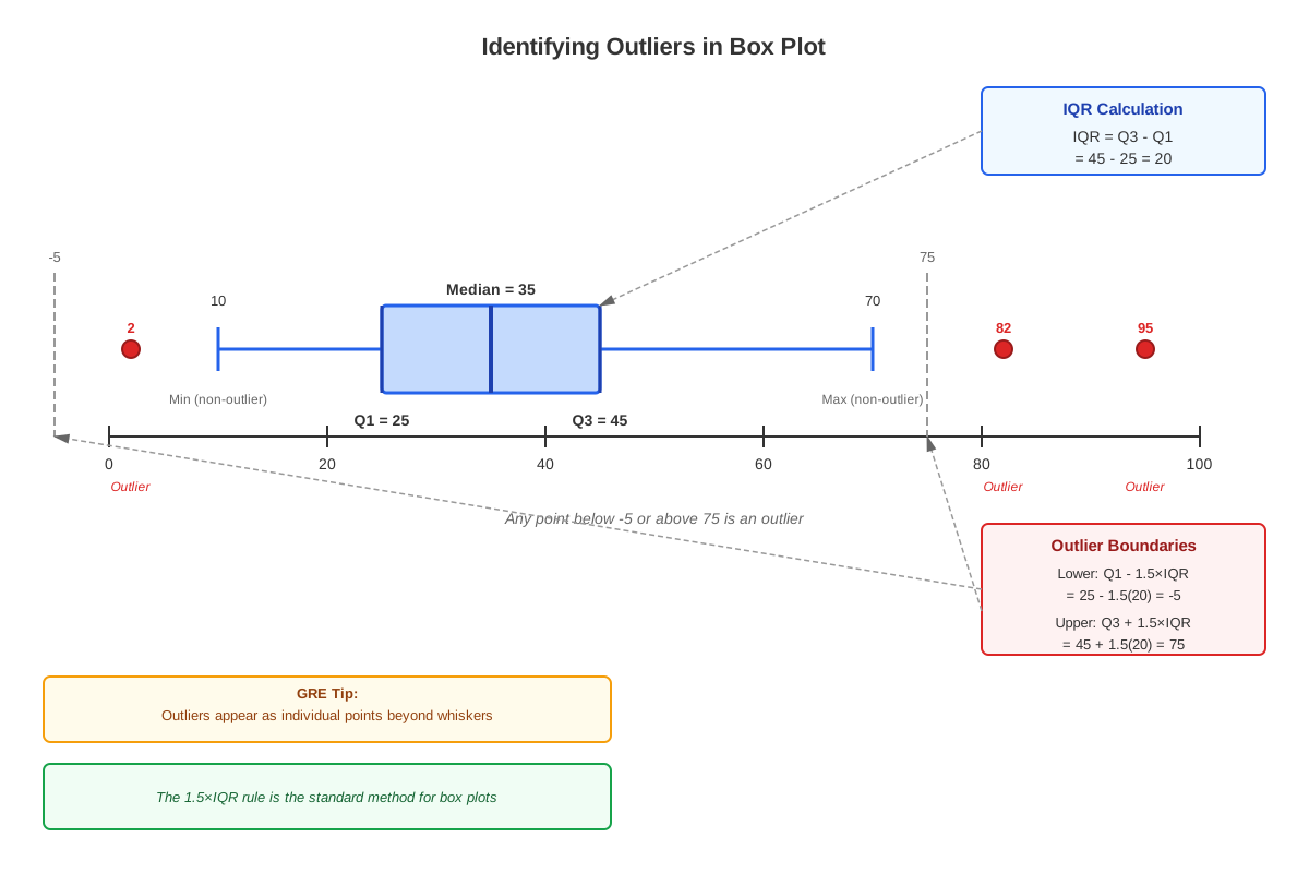
An outlier is a data point that lies an abnormal distance from other values in a dataset. While various formal statistical definitions exist (such as values more than 1.5 times the interquartile range beyond the quartiles), the GRE typically uses a more intuitive approach: outliers are values that are noticeably separated from the main cluster of data. For GRE purposes, students should recognize outliers as values that appear extreme relative to the rest of the dataset, whether presented numerically or graphically.
In numerical datasets, outliers stand out as values substantially larger or smaller than the majority of observations. For example, in the dataset {12, 15, 14, 13, 16, 15, 14, 87}, the value 87 is clearly an outlier because it differs dramatically from the cluster of values in the low teens. In graphical representations, outliers appear as isolated points separated from the main distribution—a single point far from others on a scatter plot, or individual data points beyond the whiskers of a box plot.
Impact on Mean (Arithmetic Average)
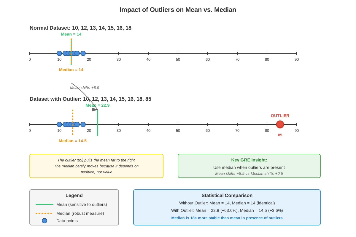
The mean is the most sensitive measure of central tendency to outliers. Because the mean is calculated by summing all values and dividing by the count, a single extreme value can dramatically shift the average. This sensitivity occurs because every data point contributes equally to the sum, regardless of how far it deviates from typical values.
Consider a dataset of five salaries: $45,000, $48,000, $50,000, $52,000, and $55,000. The mean is $50,000. If one additional salary of $500,000 is added (an outlier), the new mean becomes $125,000—a value that no longer represents a "typical" salary in the group. This dramatic shift demonstrates why the mean can be misleading when outliers are present. On the GRE, questions frequently exploit this property by asking students to compare means before and after outliers are added or removed, or to determine which measure best represents a dataset containing extreme values.
Impact on Median
The median is highly resistant to outliers, making it a robust measure of central tendency for skewed distributions. The median represents the middle value when data is arranged in order, so extreme values at either end of the distribution do not affect its position unless they change which observation occupies the middle position.
Using the salary example above, the original five salaries have a median of $50,000 (the middle value). When the $500,000 outlier is added, creating six values, the median becomes $51,000 (the average of the third and fourth values: $50,000 and $52,000). Despite the extreme outlier, the median barely changed. This stability makes the median the preferred measure when outliers are present, and the GRE frequently tests whether students recognize this property.
Impact on Mode
The mode (the most frequently occurring value) is completely unaffected by outliers unless the outlier itself appears multiple times and becomes the most frequent value. Since outliers are typically unique extreme values, they rarely influence the mode. In datasets without repeated values, there may be no mode at all, making this measure less relevant for outlier analysis on the GRE.
Impact on Range
The range (the difference between maximum and minimum values) is extremely sensitive to outliers because it depends entirely on the two most extreme values in the dataset. A single outlier at either end will dramatically increase the range, making it a poor measure of typical variability when extreme values are present.
In the dataset {12, 15, 14, 13, 16, 15, 14, 87}, the range is 87 - 12 = 75. Without the outlier, the range would be 16 - 12 = 4. This massive difference illustrates why range can be misleading in the presence of outliers. GRE questions may ask students to calculate how much the range changes when outliers are added or removed.
Outliers in Graphical Representations
Scatter plots display outliers as points that lie far from the general pattern or trend line. These isolated points may indicate unusual relationships between variables, data entry errors, or genuinely exceptional cases. On the GRE, students must recognize these visual outliers and understand how they affect correlation strength and trend line accuracy.
Box plots (box-and-whisker plots) explicitly show outliers as individual points beyond the whiskers, which typically extend to 1.5 times the interquartile range from the box edges. Any data point beyond these whiskers is conventionally marked as an outlier. GRE questions using box plots may ask students to count outliers, determine their values, or understand how they affect the overall distribution.
Histograms show outliers as isolated bars separated from the main distribution by gaps or regions of zero frequency. These visual gaps make outliers readily apparent and help students understand the shape of the distribution.
When to Consider or Exclude Outliers
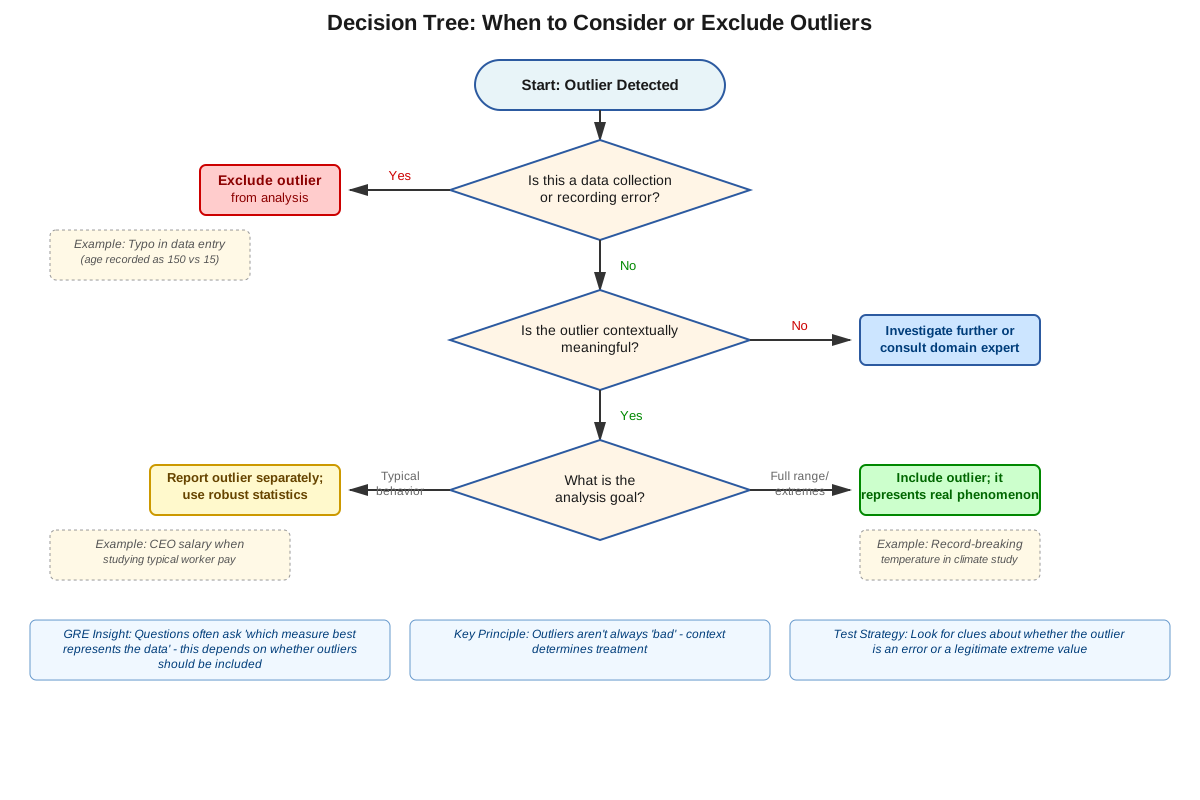
The decision to include or exclude outliers depends on their cause and the analysis purpose. Valid outliers represent genuine extreme values that provide important information about variability and should typically be retained. Examples include record-breaking performances, rare but real events, or legitimate extreme measurements.
Invalid outliers result from measurement errors, data entry mistakes, or sampling problems and should often be excluded or corrected. However, the GRE rarely asks students to make this judgment; instead, questions typically specify whether to include or exclude outliers, or they ask students to calculate statistics both ways and compare results.
Comparison Table: Statistical Measures and Outlier Sensitivity
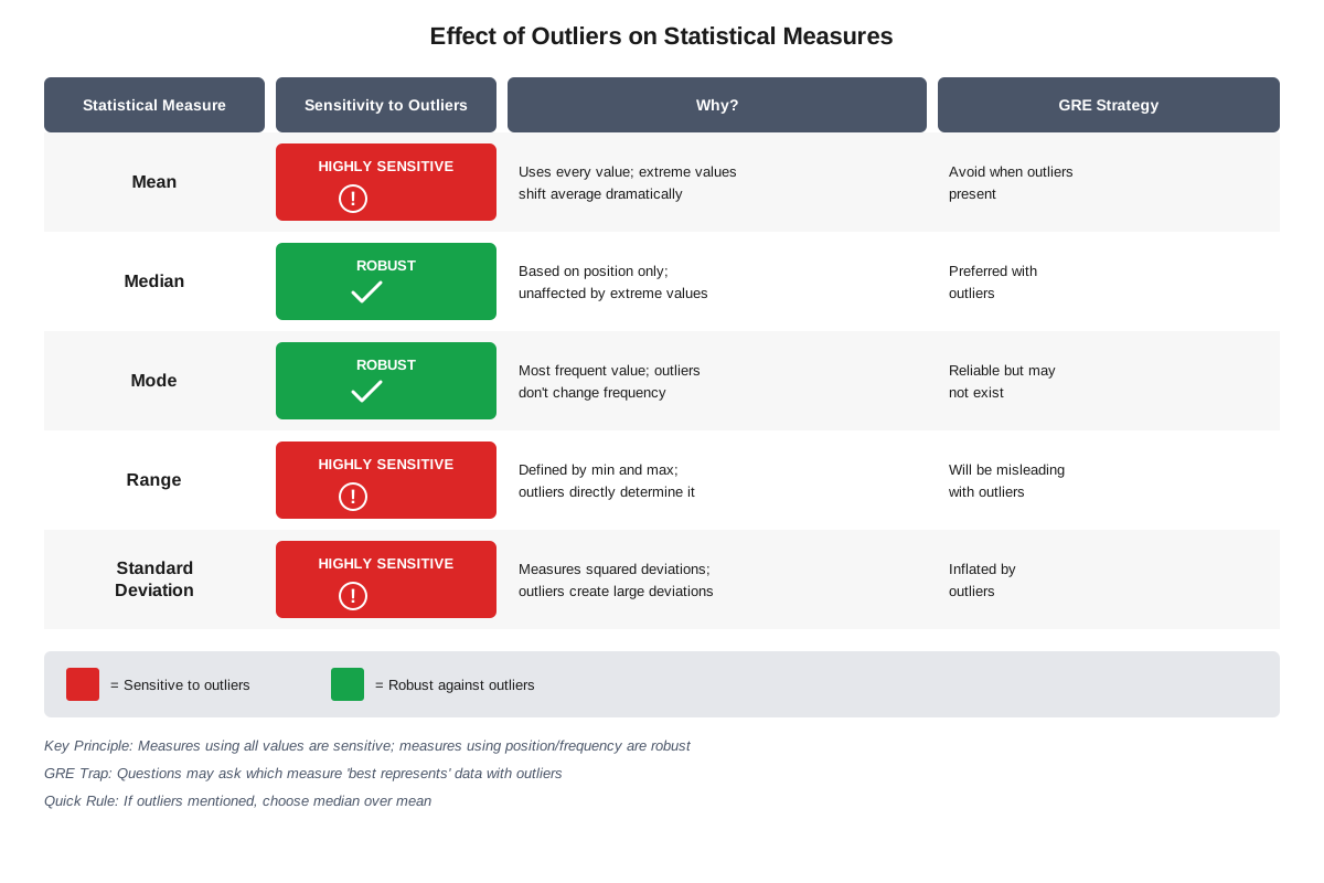
| Statistical Measure | Sensitivity to Outliers | Best Use Case |
|---|---|---|
| Mean | Very High | Symmetric distributions without outliers |
| Median | Very Low | Skewed distributions or datasets with outliers |
| Mode | None (usually) | Categorical data or identifying most common value |
| Range | Very High | Quick variability check in clean datasets |
| Standard Deviation | High | Measuring spread in symmetric distributions |
| Interquartile Range | Low | Measuring spread when outliers are present |
Concept Relationships
The concept of outliers serves as a central node connecting multiple statistical ideas. Outliers → affect → Measures of Central Tendency, with the mean being most sensitive, the median being resistant, and the mode being largely unaffected. This relationship is fundamental to understanding which summary statistic best represents a dataset.
Outliers → influence → Measures of Spread, particularly the range and standard deviation, both of which increase dramatically when extreme values are present. This connection helps students understand why the interquartile range (which excludes the most extreme quartiles) provides a more stable measure of variability.
Data Distribution Shape → determines → Outlier Impact, as symmetric distributions are more disrupted by outliers than skewed distributions where extreme values may be expected. Understanding distribution shapes helps students predict when outliers will be problematic.
Graphical Representations → reveal → Outliers, creating a bidirectional relationship where visual displays help identify extreme values, and understanding outliers improves graph interpretation. Scatter plots, box plots, and histograms each show outliers differently, requiring students to recognize various visual patterns.
Outliers → connect to → Data Quality Assessment, as extreme values may indicate measurement errors, sampling problems, or genuinely unusual phenomena. This relationship extends beyond pure calculation to analytical reasoning about data reliability.
The prerequisite concepts of mean, median, and range provide the foundation upon which outlier understanding is built, while mastery of outliers enables progression to more advanced topics like correlation analysis, regression, and statistical inference, where extreme values can significantly affect conclusions.
High-Yield Facts
⭐ The mean is the most sensitive measure of central tendency to outliers, often shifting dramatically when extreme values are added or removed.
⭐ The median is resistant to outliers, making it the preferred measure of central tendency for skewed distributions or datasets with extreme values.
⭐ A single outlier can dramatically increase the range, making range an unreliable measure of typical variability when extreme values are present.
⭐ Outliers appear as isolated points on scatter plots, separated from the main cluster or trend line.
⭐ In box plots, outliers are shown as individual points beyond the whiskers, which typically extend 1.5 times the interquartile range from the box.
- The mode is generally unaffected by outliers unless the outlier value appears multiple times and becomes the most frequent.
- Standard deviation increases when outliers are present because it measures average distance from the mean, and outliers are far from the mean.
- The interquartile range (IQR) is resistant to outliers because it measures the spread of the middle 50% of data, excluding extreme values.
- When comparing two datasets, the one with outliers will typically have a larger difference between mean and median.
- Removing an outlier that is larger than the mean will decrease the mean; removing an outlier smaller than the mean will increase the mean.
- The median can only change when an outlier's removal or addition changes which value(s) occupy the middle position(s) in the ordered dataset.
- In a dataset with a positive outlier (extremely large value), the mean will be greater than the median; with a negative outlier (extremely small value), the mean will be less than the median.
Quick check — test yourself on Outliers so far.
Try Flashcards →Common Misconceptions
Misconception: All extreme values are outliers that should be removed from analysis.
Correction: Outliers are not inherently "bad" data points. Many outliers represent genuine extreme values that provide important information about variability and should be retained. Only outliers resulting from measurement errors or data entry mistakes should be considered for removal, and the GRE typically specifies whether to include or exclude them.
Misconception: The median is always the best measure of central tendency.
Correction: While the median is resistant to outliers and preferred for skewed distributions, the mean is more appropriate for symmetric distributions without outliers because it uses all data points and has better mathematical properties for further statistical analysis. The "best" measure depends on the distribution shape and analysis purpose.
Misconception: Outliers affect all statistical measures equally.
Correction: Different measures have vastly different sensitivity to outliers. The mean and range are highly sensitive, the median and mode are resistant, and the interquartile range is moderately resistant. Understanding these differences is crucial for selecting appropriate statistics and interpreting results correctly.
Misconception: If a dataset has an outlier, the mean is always wrong or useless.
Correction: The mean is not "wrong" when outliers are present; it simply represents a different aspect of the data (the arithmetic average of all values, including extremes). The mean may be less representative of "typical" values, but it accurately reflects the sum of all observations divided by the count, which can be meaningful depending on the context.
Misconception: Outliers only occur in large datasets.
Correction: Outliers can appear in datasets of any size, including very small ones. Even a dataset with just three values can contain an outlier if one value is substantially different from the other two. The GRE frequently uses small datasets to test outlier concepts because they allow for easier calculation.
Misconception: The presence of an outlier always indicates a problem with data collection.
Correction: While some outliers result from errors, many represent genuine extreme values that occur naturally in real-world phenomena. Record-breaking performances, rare events, and exceptional cases are all valid outliers that provide valuable information about the full range of possible values.
Worked Examples
Example 1: Impact of Outliers on Mean and Median
Problem: A small company has seven employees with the following annual salaries: $42,000, $45,000, $47,000, $50,000, $52,000, $54,000, and $280,000. The CEO wants to report a "typical" salary to prospective employees. Compare the mean and median, and determine which better represents a typical employee salary.
Solution:
Step 1: Calculate the mean.
Sum of all salaries = $42,000 + $45,000 + $47,000 + $50,000 + $52,000 + $54,000 + $280,000 = $570,000
Mean = $570,000 ÷ 7 = $81,428.57
Step 2: Calculate the median.
Arrange salaries in order (already ordered): $42,000, $45,000, $47,000, $50,000, $52,000, $54,000, $280,000
With 7 values, the median is the 4th value: $50,000
Step 3: Identify the outlier.
The salary of $280,000 is clearly an outlier, substantially higher than the cluster of salaries between $42,000 and $54,000.
Step 4: Analyze which measure is more representative.
The mean of $81,428.57 is higher than six of the seven salaries, making it unrepresentative of what a typical employee earns. The median of $50,000 falls in the middle of the main cluster and better represents a typical salary.
Step 5: Verify by calculating statistics without the outlier.
Without $280,000: Sum = $290,000, Mean = $290,000 ÷ 6 = $48,333.33
The median of the remaining six values = ($47,000 + $50,000) ÷ 2 = $48,500
Conclusion: The median ($50,000) better represents a typical employee salary because it is resistant to the outlier. The mean is heavily influenced by the extreme value of $280,000, making it misleading for describing typical salaries. This example demonstrates the core principle that the median is preferred when outliers are present.
Connection to Learning Objectives: This problem requires identifying the outlier ($280,000), explaining how it affects different measures (mean shifts dramatically, median remains stable), and applying this understanding to determine which statistic is more appropriate for the given context.
Example 2: Quantitative Comparison with Outliers
Problem:
Dataset A: 10, 12, 14, 16, 18, 20
Dataset B: 10, 12, 14, 16, 18, 60
Quantity A: The median of Dataset A
Quantity B: The median of Dataset B
Compare the two quantities.
Solution:
Step 1: Identify the outlier.
Dataset B contains 60, which is an outlier compared to the cluster of values between 10 and 20. Dataset A has no outliers.
Step 2: Calculate the median of Dataset A.
Dataset A has 6 values, so the median is the average of the 3rd and 4th values.
Median A = (14 + 16) ÷ 2 = 15
Step 3: Calculate the median of Dataset B.
Dataset B also has 6 values, so the median is the average of the 3rd and 4th values.
Median B = (14 + 16) ÷ 2 = 15
Step 4: Compare the quantities.
Median A = 15
Median B = 15
The quantities are equal.
Step 5: Understand why the outlier didn't affect the median.
The outlier (60) is the largest value in Dataset B, but it doesn't change which values occupy the middle positions. The 3rd and 4th values remain 14 and 16 in both datasets, so the median is identical.
Answer: The two quantities are equal (Choice C).
Key Insight: This problem tests whether students understand that the median is resistant to outliers. Even though Dataset B has an extreme value that would dramatically increase the mean, the median remains unchanged because the middle values are the same. This is a classic GRE trap—students who assume outliers always affect all measures might incorrectly choose Quantity A or B.
Connection to Learning Objectives: This example requires recognizing when outliers are being tested (the datasets differ only in one extreme value), explaining the core principle (median resistance to outliers), and applying this knowledge to answer a Quantitative Comparison question accurately.
Exam Strategy
When approaching GRE questions involving outliers, begin by scanning the dataset or graph for extreme values that are noticeably separated from the main cluster. Look for numbers that are substantially larger or smaller than others, or points that appear isolated on graphs. This initial identification helps you anticipate which statistical measures will be most affected.
Trigger words and phrases that signal outlier questions include: "extreme value," "unusual observation," "one value is much larger/smaller," "which measure best represents typical," "most/least affected by," "resistant to extreme values," and "if the highest/lowest value is removed." Questions asking you to compare mean and median, or to calculate statistics before and after adding/removing a value, almost always involve outlier concepts.
For Quantitative Comparison questions, immediately determine whether the comparison involves measures with different outlier sensitivity. If one quantity uses the mean and another uses the median, and the dataset contains an outlier, the mean will be pulled toward the outlier while the median remains stable. This pattern appears frequently and provides a quick path to the correct answer.
When calculating the impact of outliers, use this systematic approach:
- Calculate the original statistic (mean, median, or range)
- Identify the outlier and determine if it's being added or removed
- Recalculate the statistic with the change
- Compare the before and after values to quantify the impact
For process-of-elimination, remember that answer choices suggesting the median changes dramatically due to an outlier are usually incorrect, while choices indicating the mean is unaffected by outliers are also wrong. Eliminate options that contradict the fundamental principle that mean is sensitive and median is resistant to extreme values.
Time allocation: Most outlier questions can be solved in 1.5-2 minutes. If a problem requires extensive calculation, look for shortcuts—you may only need to determine the direction of change (increase or decrease) rather than the exact value. For Data Interpretation sets with multiple questions, identify outliers in the initial graph analysis to save time on subsequent questions.
Exam Tip: If a question asks which measure "best represents" or is "most typical," and the dataset contains an outlier, the answer is almost always the median. The GRE frequently tests this specific concept.
Memory Techniques
MORSE - Remember which measures are sensitive to outliers:
- Mean - Most sensitive
- Outliers affect it
- Range - Really sensitive
- Standard deviation - Sensitive
- Except median (resistant)
"Mean is MEAN to outliers" - The mean is dramatically affected by (mean to) outliers, while the median is kind and doesn't change much.
Visual Memory Aid: Picture a tug-of-war where the mean is a person being pulled dramatically toward an outlier, while the median is a person standing firm in the middle, barely moving. This image reinforces that the mean shifts toward outliers while the median stays stable.
The 50% Rule for Median: Remember that the median represents the 50th percentile—the middle value. Since outliers are at the extremes (far from the middle), they can't directly affect the middle position unless they change which observation occupies that position. This conceptual understanding helps you remember why the median is resistant.
Range Rhyme: "Range depends on the extremes, so outliers change what range means." This simple rhyme helps you remember that range is calculated from the maximum and minimum values, making it highly sensitive to outliers.
Box Plot Boundaries: Remember "1.5 times IQR" as the standard boundary for outliers in box plots. Visualize the box (containing the middle 50% of data) with whiskers extending 1.5 times the box height in each direction, and any points beyond those whiskers are outliers.
Summary
Outliers are extreme data points that differ significantly from other observations in a dataset, and understanding their impact on statistical measures is essential for GRE success. The mean is highly sensitive to outliers and can shift dramatically when extreme values are present, while the median is resistant to outliers and remains stable, making it the preferred measure of central tendency for skewed distributions. The range is also extremely sensitive to outliers since it depends entirely on the maximum and minimum values. On the GRE, outliers appear frequently in Data Analysis questions through various formats including scatter plots, box plots, numerical datasets, and word problems. Students must be able to identify outliers visually and numerically, calculate how they affect different statistical measures, and determine which measures best represent typical values in their presence. The key to mastering this topic is understanding the differential sensitivity of statistical measures and recognizing that outliers are not inherently problematic—they simply require careful consideration when selecting and interpreting summary statistics.
Key Takeaways
- Outliers are extreme values that lie far from the main cluster of data, identifiable both numerically and graphically through their separation from typical observations.
- The mean is the most sensitive measure to outliers, shifting dramatically toward extreme values, while the median is highly resistant and remains stable.
- When a dataset contains outliers, the median typically provides a better representation of "typical" values than the mean, making it the preferred measure for skewed distributions.
- Range and standard deviation are both sensitive to outliers, increasing substantially when extreme values are present, while the interquartile range is more resistant.
- Outliers appear on the GRE in multiple formats: scatter plots (isolated points), box plots (points beyond whiskers), and numerical datasets (extreme values).
- Removing an outlier larger than the mean decreases the mean; removing an outlier smaller than the mean increases the mean, but the median changes only if the middle position(s) are affected.
- The presence of outliers does not automatically indicate data problems—many outliers represent genuine extreme values that provide important information about variability.
Related Topics
Standard Deviation and Variance: These measures of spread are sensitive to outliers, similar to the mean. Understanding how outliers inflate standard deviation builds on the concepts covered here and is essential for more advanced statistical reasoning.
Interquartile Range (IQR): This measure of spread is resistant to outliers because it focuses on the middle 50% of data. Mastering outliers provides the foundation for understanding why IQR is preferred when extreme values are present.
Box Plots and Data Visualization: Box plots explicitly show outliers as points beyond the whiskers. Understanding outliers enables deeper interpretation of these graphical representations and their statistical implications.
Correlation and Regression: Outliers can dramatically affect correlation coefficients and regression lines. The concepts learned here about extreme values extend naturally to bivariate data analysis.
Data Quality and Sampling: Determining whether outliers represent valid data or errors connects to broader questions about data collection, sampling methods, and statistical inference—topics that appear in advanced GRE questions.
Practice CTA
Now that you've mastered the core concepts of outliers and their impact on statistical measures, it's time to reinforce your understanding through active practice. Attempt the practice questions to test your ability to identify outliers, calculate their effects on different measures, and apply strategic reasoning to GRE-style problems. Use the flashcards to drill the high-yield facts until they become automatic, particularly the differential sensitivity of mean versus median. Remember, understanding outliers is not just about memorizing rules—it's about developing the analytical skills to interpret data accurately under exam conditions. Every practice question you complete strengthens your ability to recognize outlier patterns quickly and respond confidently, bringing you closer to your target GRE score. Start practicing now to transform your knowledge into exam-day success!
Sign up free to keep reading
Create a free AnvayaPrep account to finish this GRE guide on Outliers — plus flashcards and practice questions.