Overview
The normal distribution basics form a cornerstone of data analysis on the GRE Quantitative Reasoning section. This bell-shaped probability distribution appears frequently in questions involving statistics, data interpretation, and probability. Understanding the fundamental properties of the normal distribution—including its symmetry, the empirical rule (68-95-99.7 rule), and how to interpret standard deviations from the mean—is essential for quickly and accurately solving a variety of GRE problems. Questions may present data sets, ask students to estimate probabilities, or require interpretation of statistical information presented in graphs or tables.
The GRE normal distribution basics tested on the exam focus primarily on conceptual understanding rather than complex calculations. Students must recognize when data follows a normal distribution pattern, apply the empirical rule to estimate percentages of data within certain ranges, and understand the relationship between mean, median, mode, and standard deviation in normally distributed data. Unlike advanced statistics courses, the GRE does not require knowledge of z-scores, probability density functions, or advanced statistical inference—instead, it emphasizes practical interpretation and application of basic normal distribution properties.
Mastering normal distribution basics connects directly to broader Quantitative Reasoning skills including data interpretation, probability concepts, and statistical reasoning. This topic frequently appears alongside questions about measures of central tendency, variability, and data visualization. A solid grasp of normal distribution principles enables students to quickly eliminate incorrect answer choices, estimate values without extensive calculation, and confidently approach data analysis questions that constitute a significant portion of the Quantitative Reasoning section.
Learning Objectives
- [ ] Identify when Normal distribution basics is being tested
- [ ] Explain the core rule or strategy behind Normal distribution basics
- [ ] Apply Normal distribution basics to GRE-style questions accurately
- [ ] Calculate the percentage of data within 1, 2, and 3 standard deviations of the mean using the empirical rule
- [ ] Recognize the properties of symmetry in normal distributions and their implications for data interpretation
- [ ] Compare normal distributions with different means and standard deviations to understand their relative spread and center
Prerequisites
- Basic statistics concepts (mean, median, mode): Understanding measures of central tendency is essential because the normal distribution is defined by its mean, and recognizing that all three measures coincide in a perfectly normal distribution is fundamental.
- Standard deviation concept: Familiarity with standard deviation as a measure of spread is necessary because the empirical rule is expressed in terms of standard deviations from the mean.
- Percentage and probability basics: Converting between percentages, decimals, and fractions is required for interpreting the proportion of data within various ranges of a normal distribution.
- Graph interpretation skills: Reading and analyzing bell curves, histograms, and other visual representations of data is crucial for identifying normal distributions in GRE questions.
Why This Topic Matters
Normal distributions model countless real-world phenomena, from test scores and heights to measurement errors and natural variations in biological systems. In professional and academic contexts, understanding normal distribution basics enables informed decision-making about quality control, risk assessment, performance evaluation, and research interpretation. The ability to quickly estimate probabilities and understand data spread is valuable across fields including business analytics, social sciences, natural sciences, and engineering.
On the GRE, normal distribution questions appear with high frequency, typically comprising 2-4 questions per Quantitative Reasoning section. These questions most commonly appear as:
- Data interpretation problems requiring students to estimate percentages of data within specified ranges
- Comparison questions (Quantitative Comparison format) asking students to compare values or probabilities in normally distributed data sets
- Word problems presenting scenarios involving test scores, measurements, or other normally distributed variables
- Graph interpretation questions showing bell curves or histograms and asking about data characteristics
The GRE specifically tests whether students can apply the empirical rule quickly, recognize symmetry properties, and make logical inferences about data without performing complex calculations. Questions often include distractors designed to catch students who confuse standard deviations with percentages or who fail to recognize the symmetry of the distribution.
Core Concepts
The Normal Distribution Shape and Properties
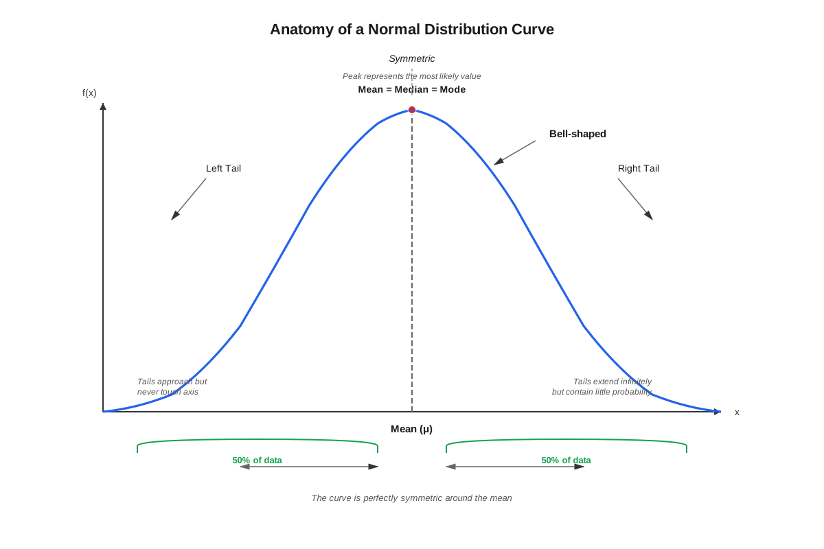
A normal distribution is a continuous probability distribution characterized by its distinctive bell-shaped curve. This symmetrical distribution is completely defined by two parameters: the mean (μ) and the standard deviation (σ). The curve is highest at the mean and decreases smoothly and symmetrically on both sides, approaching but never touching the horizontal axis.
Key properties of the normal distribution include:
- Perfect symmetry around the mean
- Mean = Median = Mode (all three measures of central tendency coincide at the center)
- The total area under the curve equals 1 (representing 100% of the data)
- Approximately 99.7% of all data falls within 3 standard deviations of the mean
- The curve is asymptotic (the tails extend infinitely without touching the x-axis)
The Empirical Rule (68-95-99.7 Rule)
The empirical rule is the most critical concept for GRE normal distribution questions. This rule states that for any normal distribution:
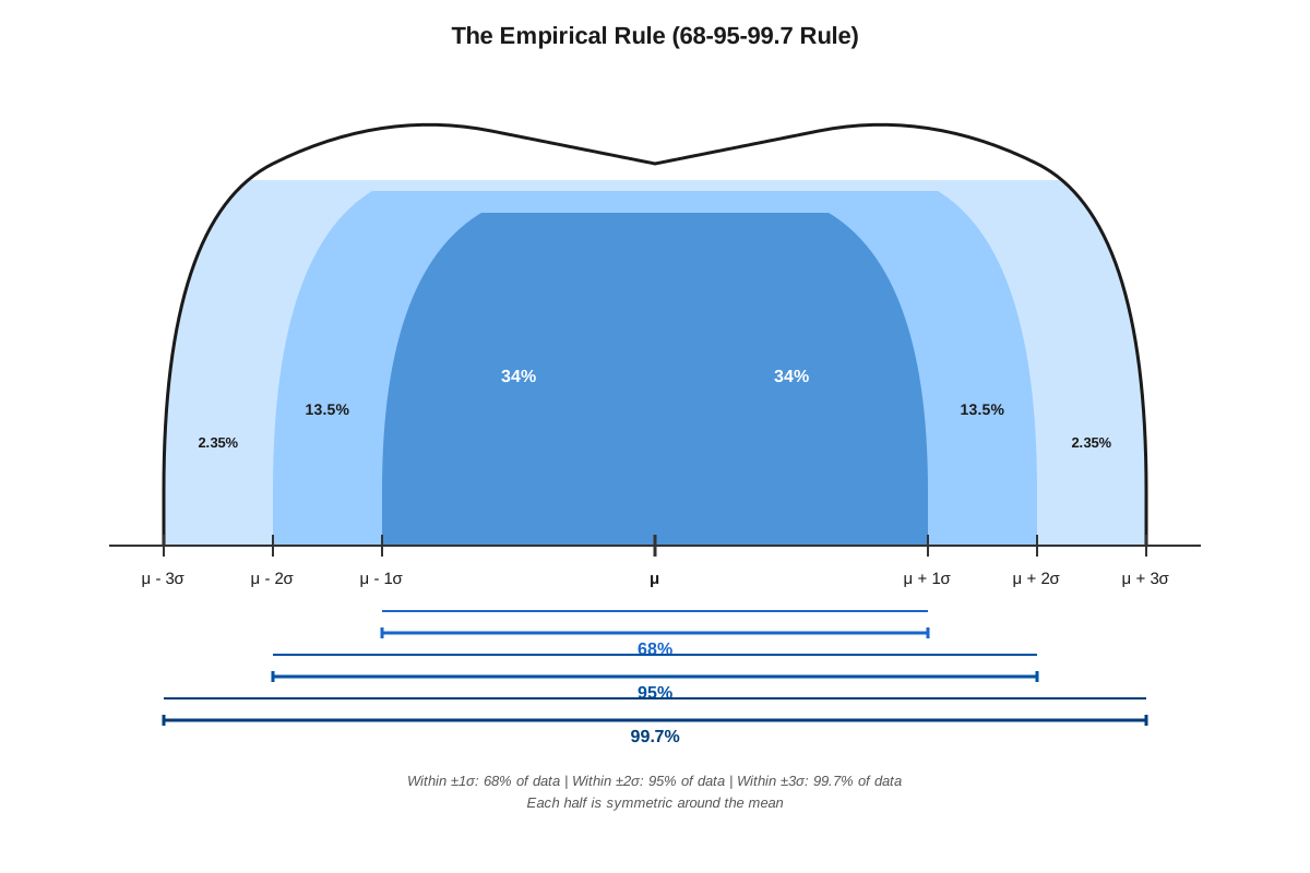
- 68% of data falls within 1 standard deviation of the mean (μ ± 1σ)
- 95% of data falls within 2 standard deviations of the mean (μ ± 2σ)
- 99.7% of data falls within 3 standard deviations of the mean (μ ± 3σ)
This rule allows rapid estimation of data percentages without complex calculations. Understanding the empirical rule means recognizing that:
- The remaining 32% (100% - 68%) of data lies beyond 1 standard deviation from the mean
- Due to symmetry, 16% lies above μ + 1σ and 16% lies below μ - 1σ
- Similarly, 2.5% lies above μ + 2σ and 2.5% lies below μ - 2σ
- Only 0.15% lies above μ + 3σ and 0.15% lies below μ - 3σ
Standard Deviation and Spread
The standard deviation (σ) measures the average distance of data points from the mean. In a normal distribution:
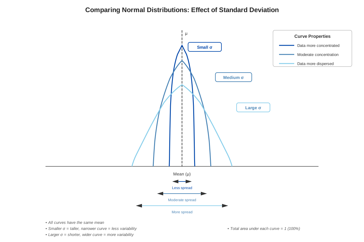
- A smaller standard deviation produces a taller, narrower bell curve (data clustered tightly around the mean)
- A larger standard deviation produces a shorter, wider bell curve (data more spread out)
- Two normal distributions can have the same mean but different standard deviations, resulting in different shapes
- Two normal distributions can have different means but the same standard deviation, resulting in identical shapes shifted horizontally
Percentiles and the Normal Distribution
Understanding percentiles in the context of normal distributions is crucial for GRE questions. Due to symmetry:
- The mean represents the 50th percentile (median)
- The 84th percentile is located at μ + 1σ (50% + 34% = 84%)
- The 16th percentile is located at μ - 1σ (50% - 34% = 16%)
- The 97.5th percentile is located at μ + 2σ
- The 2.5th percentile is located at μ - 2σ
Comparing Values in Normal Distributions
When comparing values from different normal distributions or determining relative positions:
- Calculate how many standard deviations each value is from its respective mean
- The value that is more standard deviations above its mean is relatively higher
- Use the empirical rule to estimate what percentage of data falls above or below specific values
| Range | Percentage Within | Percentage Outside | Percentage Above Upper Bound | Percentage Below Lower Bound |
|---|---|---|---|---|
| μ ± 1σ | 68% | 32% | 16% | 16% |
| μ ± 2σ | 95% | 5% | 2.5% | 2.5% |
| μ ± 3σ | 99.7% | 0.3% | 0.15% | 0.15% |
Recognizing Normal Distribution in GRE Questions
The GRE signals normal distribution questions through specific language:
- "Normally distributed"
- "Bell-shaped distribution"
- References to "standard deviations from the mean"
- Graphs showing symmetrical bell curves
- Contexts involving test scores, measurements, or natural variations
Concept Relationships
The concepts within normal distribution basics form an interconnected framework. The mean serves as the central anchor point → which determines the center of symmetry → from which standard deviations measure spread → which enables application of the empirical rule → which allows calculation of percentages and percentiles → which facilitates comparison of values across distributions.
The symmetry property connects directly to the relationship between mean, median, and mode, reinforcing prerequisite knowledge of central tendency measures. Understanding that these three measures coincide in a normal distribution helps students quickly identify when data is NOT normally distributed (when mean ≠ median).
The empirical rule builds upon the concept of standard deviation from prerequisite knowledge, transforming an abstract measure of spread into a practical tool for estimating data percentages. This rule connects to probability concepts, as percentages can be interpreted as probabilities of randomly selecting a data point within a specified range.
Percentile interpretation bridges normal distribution basics with ranking and comparison problems elsewhere in the GRE. Understanding that the 84th percentile equals μ + 1σ connects the empirical rule to practical questions about test scores, performance rankings, and data interpretation.
The relationship between different normal distributions (varying means and standard deviations) connects to comparison and data interpretation skills. Recognizing that distributions with the same shape but different centers can be directly compared through their standard deviations enables sophisticated problem-solving on Quantitative Comparison questions.
Quick check — test yourself on Normal distribution basics so far.
Try Flashcards →High-Yield Facts
⭐ In a normal distribution, exactly 68% of data falls within one standard deviation of the mean (μ ± 1σ)
⭐ In a normal distribution, exactly 95% of data falls within two standard deviations of the mean (μ ± 2σ)
⭐ The normal distribution is perfectly symmetrical around the mean, so exactly 50% of data lies above the mean and 50% below
⭐ In a normal distribution, the mean, median, and mode are all equal and located at the center of the distribution
⭐ Due to symmetry, 16% of data lies above μ + 1σ and 16% lies below μ - 1σ
- Approximately 99.7% of data in a normal distribution falls within three standard deviations of the mean
- Only 2.5% of data lies above μ + 2σ in a normal distribution
- The 84th percentile of a normal distribution is located at exactly one standard deviation above the mean
- A larger standard deviation indicates greater variability and a wider, flatter bell curve
- Two normal distributions with the same standard deviation have the same shape regardless of their means
- The total area under a normal distribution curve always equals 1 (or 100%)
- Normal distributions are asymptotic, meaning the tails approach but never touch the horizontal axis
Common Misconceptions
Misconception: The empirical rule percentages (68%, 95%, 99.7%) represent the data above the mean within each range. → Correction: These percentages represent the data within the specified range on BOTH sides of the mean. For example, 68% includes data from μ - 1σ to μ + 1σ, not just above the mean.
Misconception: A value that is 2 standard deviations above the mean is at the 95th percentile. → Correction: A value at μ + 2σ is at the 97.5th percentile, not the 95th. The 95% refers to the total percentage within ±2σ (from μ - 2σ to μ + 2σ), and due to symmetry, 2.5% lies above μ + 2σ, making it the 97.5th percentile.
Misconception: All bell-shaped distributions are normal distributions. → Correction: While normal distributions are bell-shaped, not all bell-shaped distributions are normal. A distribution must be perfectly symmetrical and follow the empirical rule precisely to be considered normal. Some distributions may appear bell-shaped but have different properties.
Misconception: The standard deviation is the same as the range of the data. → Correction: Standard deviation measures the average distance from the mean, not the total range. The range is the difference between maximum and minimum values, while standard deviation is a measure of typical spread around the center.
Misconception: If two distributions have the same mean, they have the same shape. → Correction: Two normal distributions can have identical means but completely different shapes if their standard deviations differ. The mean determines the center location, while the standard deviation determines the spread and shape.
Misconception: Exactly 100% of data falls within 3 standard deviations of the mean. → Correction: Approximately 99.7% of data falls within 3 standard deviations. While this is nearly all the data, theoretically the tails extend infinitely, so a tiny fraction (0.3%) lies beyond ±3σ.
Worked Examples
Example 1: Applying the Empirical Rule
Problem: Test scores for a standardized exam are normally distributed with a mean of 500 and a standard deviation of 100. Approximately what percentage of test-takers scored between 400 and 700?
Solution:
Step 1: Identify the given information.
- Mean (μ) = 500
- Standard deviation (σ) = 100
- We need to find the percentage between 400 and 700
Step 2: Express the boundary values in terms of standard deviations from the mean.
- Lower bound: 400 = 500 - 100 = μ - 1σ
- Upper bound: 700 = 500 + 200 = μ + 2σ
Step 3: Visualize or sketch the distribution.
The range from 400 to 700 spans from 1 standard deviation below the mean to 2 standard deviations above the mean.
Step 4: Apply the empirical rule using symmetry.
- From μ - 1σ to μ + 1σ: 68% of data
- From μ + 1σ to μ + 2σ: We need to calculate this
The empirical rule tells us:
- Within ±1σ: 68%, so 34% is between μ and μ + 1σ, and 34% is between μ - 1σ and μ
- Within ±2σ: 95%, so 47.5% is between μ and μ + 2σ
Step 5: Calculate the total percentage.
- From μ - 1σ to μ: 34%
- From μ to μ + 1σ: 34%
- From μ + 1σ to μ + 2σ: 47.5% - 34% = 13.5%
- Total: 34% + 34% + 13.5% = 81.5%
Answer: Approximately 81.5% of test-takers scored between 400 and 700.
Connection to Learning Objectives: This example demonstrates applying normal distribution basics to GRE-style questions by using the empirical rule and understanding symmetry properties.
Example 2: Quantitative Comparison with Normal Distributions
Problem:
Quantity A: The percentage of data in a normal distribution that lies between the mean and 1 standard deviation above the mean

Quantity B: The percentage of data in a normal distribution that lies more than 2 standard deviations above the meanSolution:
Step 1: Analyze Quantity A.
The empirical rule states that 68% of data falls within ±1σ of the mean. Due to symmetry, this 68% is split equally on both sides of the mean.
- Between μ and μ + 1σ: 68% ÷ 2 = 34%
Step 2: Analyze Quantity B.
The empirical rule states that 95% of data falls within ±2σ of the mean. This means 5% falls outside this range. Due to symmetry:
- Above μ + 2σ: 5% ÷ 2 = 2.5%
Step 3: Compare the quantities.
- Quantity A: 34%
- Quantity B: 2.5%
- 34% > 2.5%
Answer: Quantity A is greater.
Connection to Learning Objectives: This example shows how to identify when normal distribution basics is being tested (through references to standard deviations and percentages) and how to apply the core strategy (using the empirical rule and symmetry) to solve Quantitative Comparison questions efficiently.
Exam Strategy
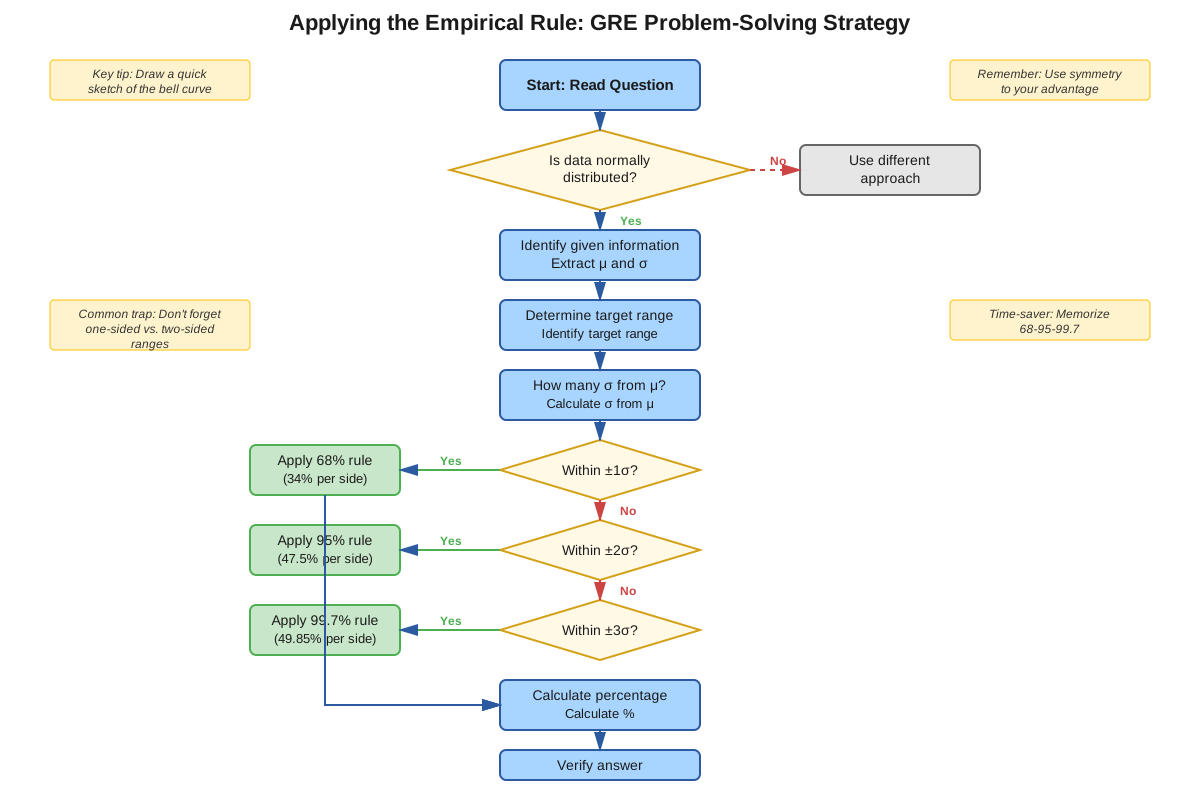
Trigger Recognition: When a GRE question mentions "normally distributed," "bell-shaped," or provides a mean and standard deviation, immediately recall the empirical rule and symmetry properties.
Approach Strategy:
- Identify the parameters: Quickly note the mean and standard deviation
- Convert values to standard deviations: Express any given values as μ ± nσ
- Apply the empirical rule: Use 68-95-99.7 to find percentages
- Use symmetry: Remember that the distribution splits 50-50 at the mean
- Estimate when exact calculation isn't needed: The GRE often accepts approximations
Process of Elimination Tips:
- Eliminate any answer choice suggesting more than 50% of data lies above (or below) the mean
- Eliminate choices that violate the empirical rule (e.g., claiming 80% of data falls within 1 standard deviation)
- Watch for answer choices that confuse "within ±nσ" with "above μ + nσ"
- Eliminate options that suggest the mean, median, and mode differ in a normal distribution
Time Allocation:
- Spend 15-20 seconds identifying that the question involves normal distribution
- Allocate 30-45 seconds applying the empirical rule
- Reserve 20-30 seconds for verification and answer selection
- If a question requires multiple steps, don't exceed 2 minutes total
Common Question Patterns:
- Direct application: "What percentage falls within X standard deviations?"
- Reverse application: "If Y% of data is above a value, how many standard deviations above the mean is it?"
- Comparison: "Which value is relatively higher in its distribution?"
- Percentile interpretation: "What percentile corresponds to μ + 1σ?"
Memory Techniques
Empirical Rule Mnemonic: "68-95-99.7: The Rule of Threes"
- Think: "6-9-9 (increasing digits) with 8-5-7 (decreasing then increasing)"
- Or remember: "Roughly 70-95-100" for quick estimation
Symmetry Visualization: Picture a perfectly balanced seesaw with the mean as the fulcrum. Everything on one side has an exact mirror on the other side.
Percentile Anchor Points:
- 50th percentile = Mean (center point)
- 84th percentile = Mean + 1SD (remember: 50 + 34 = 84)
- 16th percentile = Mean - 1SD (remember: 50 - 34 = 16)
- Think: "16-50-84" as the key percentiles for ±1σ
Standard Deviation Spread: "Small SD = Skinny curve, Large SD = Large spread" (alliteration helps memory)
Outside Percentages: "32-5-0.3" represents the percentages OUTSIDE ±1σ, ±2σ, and ±3σ respectively
- Remember: 100 - 68 = 32, 100 - 95 = 5, 100 - 99.7 = 0.3
Summary
Normal distribution basics constitute essential knowledge for GRE Quantitative Reasoning success. The normal distribution is a symmetrical, bell-shaped probability distribution completely defined by its mean and standard deviation. The empirical rule (68-95-99.7) provides the foundation for solving most GRE questions on this topic: 68% of data falls within one standard deviation of the mean, 95% within two standard deviations, and 99.7% within three standard deviations. Perfect symmetry around the mean ensures that the mean, median, and mode coincide, and that exactly 50% of data lies on each side of the center. Understanding how to express values in terms of standard deviations from the mean, apply the empirical rule to calculate percentages, and use symmetry to find percentages in specific ranges enables students to solve normal distribution questions quickly and accurately. The GRE tests conceptual understanding rather than complex calculations, emphasizing the ability to recognize when normal distribution principles apply and to make logical inferences about data characteristics.
Key Takeaways
- The empirical rule (68-95-99.7) is the single most important concept for GRE normal distribution questions
- Normal distributions are perfectly symmetrical around the mean, with mean = median = mode
- Always express values in terms of standard deviations from the mean (μ ± nσ) to apply the empirical rule
- Use symmetry to calculate percentages: if 68% falls within ±1σ, then 16% lies above μ + 1σ and 16% below μ - 1σ
- The 84th percentile corresponds to one standard deviation above the mean (μ + 1σ)
- Standard deviation determines the spread: larger standard deviation means wider, flatter curve
- GRE questions test conceptual understanding and estimation rather than precise statistical calculations
Related Topics
Z-scores and Standardization: While not heavily tested on the GRE, understanding how to standardize normal distributions by converting to z-scores builds on normal distribution basics and appears occasionally in advanced data analysis questions.
Probability and Distributions: Normal distribution basics provide the foundation for understanding other probability distributions and more advanced statistical concepts that may appear in graduate-level coursework.
Data Interpretation and Graphs: Mastering normal distribution basics enhances the ability to interpret histograms, frequency distributions, and other graphical representations of data that appear throughout the Quantitative Reasoning section.
Measures of Spread: Understanding standard deviation in the context of normal distributions deepens comprehension of variance, range, and interquartile range as measures of data variability.
Hypothesis Testing Concepts: Though beyond the GRE scope, normal distribution basics form the foundation for statistical inference, confidence intervals, and hypothesis testing encountered in graduate research and coursework.
Practice CTA
Now that you've mastered the core concepts of normal distribution basics, it's time to solidify your understanding through active practice. Attempt the practice questions to test your ability to apply the empirical rule, recognize symmetry properties, and solve GRE-style problems efficiently. Use the flashcards to reinforce the key facts, percentages, and relationships you'll need to recall quickly on test day. Remember: understanding the concepts is just the first step—consistent practice transforms knowledge into the automatic, confident problem-solving skills that lead to top GRE scores. You've built a strong foundation; now strengthen it through deliberate practice!
Sign up free to keep reading
Create a free AnvayaPrep account to finish this GRE guide on Normal distribution basics — plus flashcards and practice questions.