Optimization basics

Overview

Optimization basics refers to a category of mathematical problems that require finding the maximum or minimum value of a quantity given certain constraints. On the GRE Quantitative Reasoning section, these problems typically involve real-world scenarios where test-takers must determine the best possible outcome—whether that means maximizing profit, minimizing cost, finding the largest area with limited materials, or identifying the optimal dimensions of a geometric figure. Unlike pure algebraic manipulation, optimization problems demand strategic thinking about relationships between variables and how changes in one quantity affect another.

Understanding GRE optimization basics is essential because these questions appear regularly on the exam and test multiple mathematical competencies simultaneously. They combine algebraic reasoning, geometric principles, and logical problem-solving in ways that distinguish high-scoring test-takers from average performers. Optimization questions often appear deceptively simple but contain subtle constraints that must be carefully identified and applied. The GRE uses optimization problems to assess whether students can translate verbal descriptions into mathematical relationships, manipulate those relationships strategically, and recognize when a solution represents a true maximum or minimum.

Within the broader Quantitative Reasoning framework, optimization basics connects directly to algebra (setting up equations and inequalities), geometry (area, perimeter, and volume relationships), and arithmetic (working with rates, ratios, and proportions). These problems also reinforce critical thinking skills tested throughout the GRE: identifying relevant information, eliminating extraneous details, and systematically testing possibilities. Mastery of optimization basics provides a foundation for tackling complex word problems and demonstrates the mathematical maturity that graduate programs value.

Learning Objectives

• [ ] Identify when Optimization basics is being tested
• [ ] Explain the core rule or strategy behind Optimization basics
• [ ] Apply Optimization basics to GRE-style questions accurately
• [ ] Translate verbal optimization scenarios into mathematical expressions and constraints
• [ ] Distinguish between local and global maxima/minima in discrete and continuous contexts
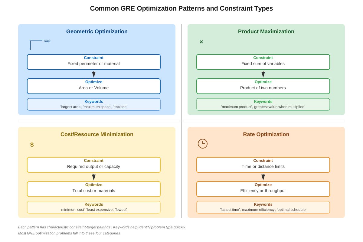
• [ ] Recognize common optimization patterns (area-perimeter trade-offs, product maximization, cost minimization)
• [ ] Verify that proposed solutions satisfy all stated constraints

Prerequisites

• Algebraic manipulation: Ability to solve equations, substitute variables, and work with expressions is fundamental to setting up and solving optimization relationships
• Basic geometry formulas: Knowledge of area, perimeter, volume, and surface area formulas enables translation of geometric optimization problems into solvable equations
• Understanding of inequalities: Recognizing constraints and valid solution ranges requires comfort with inequality notation and solution sets
• Function behavior: Basic understanding of how changing one variable affects another helps identify maximum and minimum values
• Word problem translation: Skill in converting verbal descriptions into mathematical notation is the critical first step in all optimization problems

Why This Topic Matters

Optimization problems represent real-world decision-making scenarios that resonate across business, engineering, economics, and natural sciences. From a company determining the production level that maximizes profit to an architect designing a building with maximum interior space using minimum materials, optimization thinking pervades professional problem-solving. The GRE includes these questions because graduate programs value students who can identify constraints, model relationships mathematically, and determine optimal solutions—skills essential for research design, resource allocation, and analytical reasoning in academic contexts.

On the GRE Quantitative Reasoning section, optimization questions appear with moderate to high frequency, typically comprising 2-4 questions per exam. They most commonly appear as word problems in both Quantitative Comparison and Problem Solving formats. The exam particularly favors optimization scenarios involving geometric figures (maximizing area with fixed perimeter), number relationships (finding two numbers with a given sum that maximize their product), and practical situations (minimizing cost or time). These questions often carry medium to high difficulty ratings because they require multi-step reasoning and integration of multiple mathematical concepts.

Common exam presentations include: "What dimensions maximize the area of a rectangle with perimeter 40?" or "A farmer has 200 feet of fencing to enclose a rectangular plot. What is the maximum area?" or "What is the minimum value of the expression x² + 6x + 10?" The GRE also embeds optimization within data interpretation questions, asking test-takers to identify maximum or minimum values from tables or graphs. Recognizing the optimization framework quickly—even when the word "maximum" or "minimum" doesn't explicitly appear—is a crucial test-taking skill.

Core Concepts

Fundamental Optimization Framework

The core of optimization basics involves three essential components: the objective function (what you're trying to maximize or minimize), the constraints (limitations or requirements), and the feasible region (all possible solutions that satisfy the constraints). Every optimization problem requires identifying these three elements before attempting a solution. The objective function might be area, cost, profit, time, or any measurable quantity. Constraints typically involve fixed resources (limited fencing, fixed budget, specific dimensions) or required relationships (sum must equal a certain value, one dimension must be twice another).

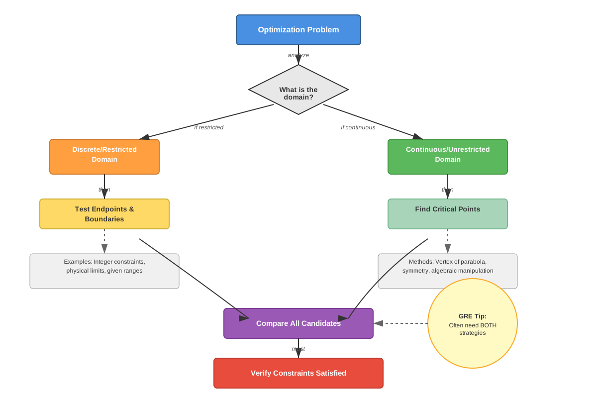
For GRE purposes, optimization problems fall into two broad categories: discrete optimization (choosing from a finite set of possibilities) and continuous optimization (finding optimal values along a continuous range). Discrete problems might ask "Which of these five production levels maximizes profit?" while continuous problems ask "What value of x minimizes this expression?" The solution strategies differ significantly between these types.

Algebraic Optimization Strategies

When optimizing algebraic expressions, the primary technique involves expressing the quantity to be optimized as a function of a single variable, then finding the maximum or minimum value. For quadratic expressions in the form ax² + bx + c, the vertex represents either a maximum (when a < 0) or minimum (when a > 0). The x-coordinate of the vertex occurs at x = -b/(2a), and substituting this value back into the expression yields the optimal value.

For example, to minimize f(x) = x² - 8x + 20, recognize that a = 1 (positive), so the parabola opens upward and has a minimum. The minimum occurs at x = -(-8)/(2·1) = 4, and the minimum value is f(4) = 16 - 32 + 20 = 4. This technique applies to any problem that can be reduced to a quadratic expression.

Another powerful algebraic strategy involves the AM-GM inequality (Arithmetic Mean-Geometric Mean inequality), which states that for positive numbers, their arithmetic mean is always greater than or equal to their geometric mean. This principle implies that for two positive numbers with a fixed sum, their product is maximized when the numbers are equal. Conversely, for two positive numbers with a fixed product, their sum is minimized when the numbers are equal.

Geometric Optimization Patterns

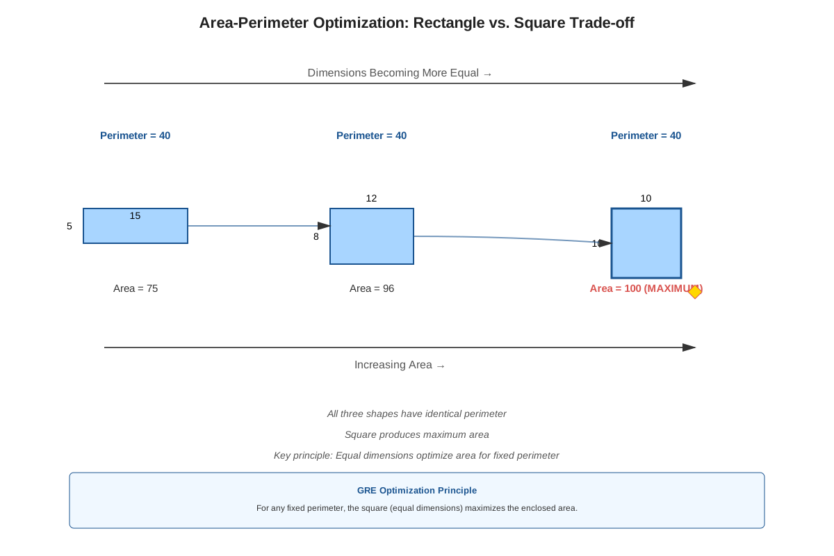
Geometric optimization problems on the GRE frequently involve area-perimeter relationships. A fundamental principle: among all rectangles with a given perimeter, the square has the maximum area. For a fixed perimeter P, the rectangle with dimensions P/4 by P/4 (a square) maximizes area. Conversely, among all rectangles with a given area, the square has the minimum perimeter.

Consider this relationship mathematically: For a rectangle with perimeter P, if one side is x, the other side is (P/2 - x). The area A = x(P/2 - x) = Px/2 - x². This is a quadratic function with a = -1 (negative), so it has a maximum. Using the vertex formula: x = -P/2 / (2·(-1)) = P/4. Thus, both dimensions equal P/4, confirming the square maximizes area.

Three-dimensional optimization follows similar principles. Among all rectangular boxes with a given surface area, the cube has maximum volume. Among all boxes with given volume, the cube has minimum surface area. These patterns appear regularly on the GRE, often disguised within practical scenarios about containers, packages, or enclosures.

Constraint-Based Optimization

Many GRE optimization problems provide explicit constraints that limit the feasible solutions. The key strategy involves using constraints to eliminate variables, reducing the problem to a single-variable optimization. For instance, if told "two positive numbers sum to 20" and asked to maximize their product, use the constraint x + y = 20 to write y = 20 - x, then express the product as P = x(20 - x) = 20x - x², which can be optimized using vertex techniques.

Boundary analysis is crucial when constraints create a limited feasible region. The optimal value might occur at an interior point (where calculus-based techniques would find it) or at a boundary point (an endpoint of the feasible range). On the GRE, always check boundary values. If asked to maximize f(x) = -x² + 10x for 0 ≤ x ≤ 8, find both the vertex (x = 5, giving f(5) = 25) and the boundary values (f(0) = 0, f(8) = 16). The maximum is 25 at the interior point x = 5.

Testing Critical Values

For discrete optimization or when dealing with integer constraints, systematic testing of critical values often provides the most efficient solution path. Critical values include: endpoints of the feasible range, integer values near the theoretical optimum, and values where the expression changes behavior. Rather than attempting complex algebraic manipulation, testing 3-5 strategic values often reveals the answer quickly.

This approach proves especially valuable for Quantitative Comparison questions. If asked to compare the maximum value of x(10-x) for positive integers x with some quantity, test x = 4, 5, and 6 (values near the middle of the range 0 to 10). Calculate: f(4) = 24, f(5) = 25, f(6) = 24. The maximum is 25, achieved at x = 5.

Concept Relationships

The concepts within optimization basics form a hierarchical structure. The fundamental framework (identifying objective function, constraints, and feasible region) serves as the foundation for all other techniques. This framework leads directly to variable elimination, where constraints are used to express the objective function in terms of a single variable. Once expressed as a single-variable function, the problem branches into either algebraic optimization (using vertex formulas, AM-GM inequality, or completing the square) or geometric optimization (applying area-perimeter principles or volume-surface area relationships).

Both algebraic and geometric approaches converge at the critical value testing stage, where proposed optimal values must be verified against constraints and compared with boundary values. This verification step connects back to the fundamental framework, ensuring the solution lies within the feasible region.

Optimization basics builds directly on prerequisite knowledge: algebraic manipulation enables variable elimination and expression simplification; geometric formulas provide the relationships needed for spatial optimization; inequality understanding helps identify feasible regions; and function behavior knowledge supports recognizing maxima and minima. Looking forward, optimization basics provides essential preparation for more advanced topics in data analysis, probability optimization, and complex multi-constraint problems.

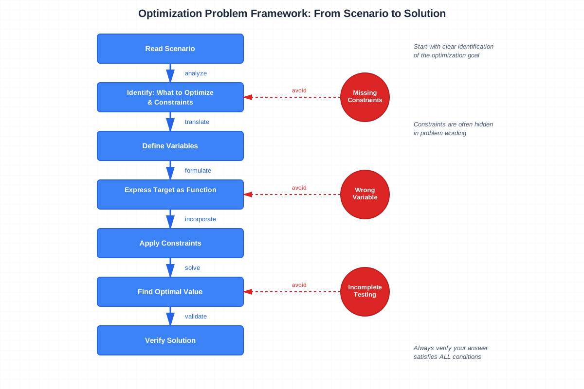
The relationship map: Identify Problem Type → Extract Constraints → Eliminate Variables → Express as Single-Variable Function → Apply Optimization Technique (Vertex Formula/AM-GM/Geometric Principle) → Test Critical Values → Verify Against Constraints → Confirm Maximum/Minimum.

High-Yield Facts

• ⭐ For a quadratic function f(x) = ax² + bx + c, the vertex (optimal value) occurs at x = -b/(2a); this is a minimum when a > 0 and a maximum when a < 0
• ⭐ Among all rectangles with a given perimeter, the square has the maximum area
• ⭐ For two positive numbers with a fixed sum, their product is maximized when the numbers are equal
• ⭐ For two positive numbers with a fixed product, their sum is minimized when the numbers are equal
• ⭐ Always check boundary values of the feasible region; the optimal value may occur at an endpoint rather than an interior point
• The area of a rectangle with perimeter P is maximized when both dimensions equal P/4
• Among all rectangular boxes with fixed surface area, the cube has maximum volume
• When optimizing products of variables with a fixed sum S, the maximum product is (S/2)² when there are two variables
• Optimization problems often require expressing one variable in terms of another using constraint equations
• Integer constraint problems may have optimal values different from continuous optimization solutions
• The expression x² + y² is minimized (for fixed x + y) when x = y
• For a fixed perimeter, circular shapes enclose more area than polygonal shapes
• Completing the square transforms any quadratic into vertex form, revealing the optimal value immediately
• Optimization problems frequently test whether students recognize that "at least" and "at most" create inequality constraints
• When multiple constraints exist, the feasible region is the intersection of all individual constraint regions

Common Misconceptions

Misconception: The maximum or minimum always occurs at the vertex of a parabola, regardless of constraints. → Correction: When the feasible region is restricted (e.g., x must be between 2 and 8), the optimal value might occur at a boundary point rather than the vertex. Always evaluate the function at both the vertex and all boundary points, then compare.

Misconception: To maximize the area of a rectangle, make one dimension as large as possible. → Correction: Maximizing area with a fixed perimeter requires balancing the dimensions. Making one dimension very large forces the other to be very small, reducing total area. The square (equal dimensions) maximizes area for a given perimeter.

Misconception: If two numbers sum to S, their maximum product is S². → Correction: The maximum product is (S/2)², which occurs when both numbers equal S/2. For example, if x + y = 10, the maximum product is 25 (when x = y = 5), not 100.

Misconception: Optimization problems always require calculus or advanced techniques. → Correction: GRE optimization problems are designed to be solved using algebra, geometric principles, and strategic testing. Recognizing standard patterns (area-perimeter relationships, sum-product optimization) often provides immediate solutions.

Misconception: The word "optimize" or "maximum/minimum" must appear for a problem to be an optimization question. → Correction: Many optimization problems are disguised with phrases like "what is the greatest possible," "what is the least value," "what dimensions give the largest," or "find the best arrangement." Recognizing these as optimization triggers is essential.

Misconception: When optimizing with integer constraints, simply round the continuous optimal value to the nearest integer. → Correction: Rounding doesn't always give the integer optimum. For example, if the continuous maximum of f(x) = -x² + 7x occurs at x = 3.5, you must test both f(3) and f(4) to determine which integer gives the true maximum. In this case, f(3) = 12 and f(4) = 12, so both integers are optimal.

Misconception: Larger perimeter always means larger area. → Correction: Perimeter and area are independent. A rectangle with dimensions 1 × 9 has perimeter 20 and area 9, while a rectangle with dimensions 4 × 6 has perimeter 20 and area 24. Different shapes with the same perimeter can have vastly different areas.

Misconception: In optimization problems, all given information must be used. → Correction: Some optimization problems include extraneous information to test whether students can identify relevant constraints. Focus on information that directly relates to the quantity being optimized and the constraints limiting possible solutions.

Worked Examples

Example 1: Geometric Optimization with Perimeter Constraint

Problem: A farmer has 80 meters of fencing to enclose a rectangular garden. What is the maximum area the garden can have?

Solution:

Step 1: Identify the optimization framework

• Objective function: Maximize area (A)
• Constraint: Perimeter = 80 meters
• Variables: length (l) and width (w)

Step 2: Express the constraint mathematically

The perimeter of a rectangle is P = 2l + 2w = 80, which simplifies to l + w = 40.

Step 3: Eliminate one variable

From the constraint, w = 40 - l. This allows us to express area in terms of a single variable.

Step 4: Express the objective function as a single-variable equation

Area A = l × w = l(40 - l) = 40l - l²

Step 5: Recognize this as a quadratic and find the vertex

A = -l² + 40l is a quadratic with a = -1 (negative), so it opens downward and has a maximum.

The vertex occurs at l = -b/(2a) = -40/(2(-1)) = 40/2 = 20 meters.

Step 6: Find the corresponding width

w = 40 - l = 40 - 20 = 20 meters

Step 7: Calculate the maximum area

A = l × w = 20 × 20 = 400 square meters

Step 8: Verify the solution

Check that the perimeter constraint is satisfied: 2(20) + 2(20) = 80 ✓

Note that the optimal shape is a square, confirming the principle that squares maximize area for a given perimeter.

Answer: The maximum area is 400 square meters.

Connection to learning objectives: This problem demonstrates identifying optimization (maximizing area), applying the core strategy (using constraints to create a single-variable quadratic, then finding the vertex), and verifying the solution satisfies all constraints.

Example 2: Product Optimization with Sum Constraint

Problem: Two positive numbers have a sum of 24. What is the maximum possible value of their product?

Solution:

Step 1: Define variables and identify the framework

Let the two numbers be x and y.

• Objective: Maximize P = xy (the product)
• Constraint: x + y = 24
• Additional constraint: x, y > 0 (both positive)

Step 2: Use the constraint to eliminate one variable

From x + y = 24, we get y = 24 - x

Step 3: Express the product as a function of one variable

P = x(24 - x) = 24x - x²

Step 4: Identify this as a quadratic and find the maximum

P = -x² + 24x has a = -1 (negative), so the parabola opens downward with a maximum.

The maximum occurs at x = -b/(2a) = -24/(2(-1)) = 12

Step 5: Find the other number

y = 24 - x = 24 - 12 = 12

Step 6: Calculate the maximum product

P = xy = 12 × 12 = 144

Step 7: Verify using the AM-GM principle

This result confirms the principle that for two numbers with a fixed sum, the product is maximized when the numbers are equal. Both numbers equal 24/2 = 12.

Step 8: Check boundary behavior

Consider extreme cases: if x = 1, then y = 23, and P = 23 (much less than 144). If x = 23, then y = 1, and P = 23. The interior solution (x = y = 12) clearly gives the maximum.

Answer: The maximum product is 144.

Connection to learning objectives: This example shows recognizing a classic optimization pattern (sum-product relationship), applying algebraic optimization techniques (vertex formula), and understanding the AM-GM principle that underlies many GRE optimization problems.

Exam Strategy

When approaching GRE optimization questions, begin by identifying trigger phrases that signal optimization: "maximum," "minimum," "greatest possible," "least value," "largest area," "smallest perimeter," "optimal," "best," or "most efficient." These phrases indicate that you need to find an extreme value rather than simply calculate a specific quantity.

Systematic approach for optimization questions:

1. Read carefully to identify what is being optimized (area, cost, product, sum, etc.) and what constraints limit the solution
2. Define variables clearly and write down the constraint equations
3. Eliminate variables using constraints until the objective function depends on a single variable
4. Recognize the mathematical form (quadratic, linear, geometric relationship)
5. Apply the appropriate technique (vertex formula, AM-GM, geometric principle, or systematic testing)
6. Check boundary values if the feasible region is restricted
7. Verify the answer satisfies all constraints and makes logical sense

For Quantitative Comparison questions involving optimization, determine whether you need the exact optimal value or just need to compare it with another quantity. Sometimes recognizing that "the maximum is greater than X" is sufficient without calculating the precise maximum. Use estimation and boundary testing to make comparisons efficiently.

Time management: Optimization problems typically require 1.5-2.5 minutes. If algebraic setup becomes complex after 45 seconds, switch to strategic testing of values. For problems with integer constraints, testing 4-5 values near the expected optimum often proves faster than algebraic manipulation.

Process of elimination tips: In multiple-choice optimization problems, extreme answer choices (very large or very small values) are often incorrect unless the problem involves boundary optimization. The optimal value typically lies in the middle range of possibilities. For geometric optimization, answers that represent squares or cubes are often correct due to the symmetry principles underlying optimization.

Red flags to watch for: Problems that seem to have insufficient information often require recognizing a standard optimization principle (like squares maximizing area). Questions with multiple constraints require careful attention to ensure the proposed solution satisfies all conditions. Be especially careful with "at least" and "at most" language, which creates inequality constraints that may force boundary solutions.

Memory Techniques

VERTEX mnemonic for quadratic optimization:

• Variable elimination first
• Express as single-variable quadratic
• Recognize the sign of a (positive = minimum, negative = maximum)
• Take x = -b/(2a) to find optimal x-value
• Evaluate the function at this x-value
• X-amine boundary values if constraints exist

"Square is Supreme" principle: For geometric optimization with perimeter constraints, remember that squares maximize area and cubes maximize volume. Visualize a rectangle being "pulled" into a square shape to increase area.

"Equal is Optimal" rule: When optimizing products with fixed sums or sums with fixed products, the extreme value occurs when the variables are equal. Visualize a see-saw balanced in the middle.

COVE framework for approaching any optimization problem:

• Constraints: Identify all limitations
• Objective: What are you maximizing or minimizing?
• Variables: Define and eliminate to get one variable
• Extreme: Find the maximum or minimum value

Visualization technique: For area-perimeter problems, imagine a fixed-length string forming different rectangles. As you make the shape more "square-like," the enclosed area grows. This mental image reinforces why squares optimize area.

Boundary check acronym - VEB: Always check Vertex, Endpoints, and Boundaries before finalizing your answer.

Summary

Optimization basics encompasses the strategies and techniques for finding maximum or minimum values of quantities subject to constraints. The fundamental approach involves identifying the objective function (what to optimize), extracting constraints (limitations on possible solutions), eliminating variables to create a single-variable expression, and applying appropriate optimization techniques. For quadratic functions, the vertex formula x = -b/(2a) locates optimal values. For geometric problems, recognizing that squares maximize area with fixed perimeter and that equal values optimize sum-product relationships provides immediate solutions. GRE optimization problems require translating verbal descriptions into mathematical relationships, systematically testing critical values, and verifying that solutions satisfy all constraints. Success depends on recognizing standard patterns (area-perimeter trade-offs, sum-product optimization, boundary analysis), applying algebraic manipulation efficiently, and checking both interior optimal points and boundary values. These problems integrate algebra, geometry, and logical reasoning, making them high-value questions that distinguish strong quantitative performers. Mastery requires understanding core principles, practicing pattern recognition, and developing systematic solution approaches that balance algebraic precision with strategic testing.

Key Takeaways

• Optimization problems require identifying three elements: the objective function (what to optimize), constraints (limitations), and the feasible region (valid solutions)
• For quadratic expressions ax² + bx + c, the optimal value occurs at x = -b/(2a); this is a minimum when a > 0 and maximum when a < 0
• Among rectangles with fixed perimeter, the square has maximum area; among rectangles with fixed area, the square has minimum perimeter
• For two positive numbers with fixed sum, their product is maximized when the numbers are equal (AM-GM principle)
• Always check boundary values of the feasible region; the optimal value may occur at an endpoint rather than at the vertex
• Use constraints to eliminate variables, reducing multi-variable problems to single-variable optimization
• Strategic testing of critical values (endpoints, integers near the theoretical optimum) often provides faster solutions than complex algebra

Related Topics

Advanced Optimization with Multiple Constraints: Building on optimization basics, this topic explores problems with two or more simultaneous constraints, requiring systems of equations and inequality analysis. Mastering basic optimization provides the foundation for handling these more complex scenarios.

Quadratic Functions and Parabolas: Deep understanding of quadratic behavior, including vertex form, axis of symmetry, and transformations, enhances optimization problem-solving. The vertex formula used in optimization derives from comprehensive quadratic function analysis.

Inequalities and Feasible Regions: Advanced study of linear and nonlinear inequalities expands the constraint-handling techniques introduced in optimization basics, particularly for problems involving "at least" and "at most" conditions.

Geometric Applications: Further exploration of area, perimeter, volume, and surface area relationships in two and three dimensions extends the geometric optimization patterns, including optimization with circles, triangles, and composite figures.

Rate and Work Problems: Many rate problems involve optimization elements (minimizing time, maximizing efficiency), and the variable elimination techniques from optimization basics apply directly to these scenarios.

Practice CTA

Now that you've mastered the core concepts of optimization basics, it's time to reinforce your understanding through active practice. Attempt the practice questions to apply these strategies to GRE-style problems, testing your ability to recognize optimization scenarios, set up equations efficiently, and find optimal values accurately. Use the flashcards to drill the high-yield facts and formulas until they become automatic. Remember: optimization problems reward systematic thinking and pattern recognition—skills that improve dramatically with focused practice. Each problem you solve strengthens your ability to identify optimization triggers and apply the right technique quickly. You're building the problem-solving expertise that leads to top GRE scores!